This site uses analytics to measure page views and engagement.
Py
Course Assistant
Computational Business Models
Ask me anything about the course or python code. Please note that AI tools can make mistakes, so always double-check responses against the course materials and your own work.
What is a local optimum?
Explain hill climbing
How does simulated annealing work?
What is a fitness function?
Pseudocode for a genetic algorithm
Why use np.random.seed()?
Benchmark Optimization Problems
Author
Pamela Schlosser
In optimization research, benchmark problems serve as standardized test beds that allow algorithm designers to compare performance, uncover strengths and weaknesses, and drive methodological innovation.
Overview of Problems
OneMax Problem: The OneMax problem is widely used as a benchmark in evolutionary algorithms to test how well algorithms can evolve a binary string towards an optimal solution (a string of all 1s). It is simple and useful for evaluating basic evolutionary or heuristic search methods.
Knapsack Problem: The Knapsack problem is another classic benchmark problem in optimization, particularly for combinatorial algorithms problems (COPs), or an algorithm designed to solve problems involving discrete structures. Variants such as the 0/1 Knapsack and Fractional Knapsack are commonly used to evaluate algorithms like dynamic programming, greedy algorithms, and evolutionary methods.
Ackley Function: The Ackley function is a well-known continuous optimization benchmark problem. It is often used to test optimization algorithms’ ability to handle multi-modal functions with many local minima. Algorithms like simulated annealing and genetic algorithms are frequently evaluated using this function.
Schaffer Min-Min Problem: The Schaffer Min-Min is a well-known benchmark in multi-objective optimization. It provides a simple yet effective test case for algorithms that need to identify Pareto-optimal solutions in multi-objective spaces.
These benchmark problems are critical for testing and comparing the performance of optimization algorithms, especially in research and development of new heuristic methods.
Discrete Optimization Problems
OneMax Problem
In evolutionary algorithms, the OneMax problem serves as a simple test problem where the goal is to evolve a population of binary strings towards the optimal solution (a string of all 1s). The fitness function is used to evaluate the quality of each candidate solution in the population.
Fitness Function: Imagine life had a personal ‘fitness function’ just for you. What variables would you include in it, and how would you weigh them? If 0 meant that you were unable to satisfy that goal, and 1 meant that you were able to satisfy that goal, wouldn’t you want all 1s.
One Max Formula
Binary String: A binary string is generated using NumPy’s randint function, which creates a list of 0s and 1s.
Fitness Function: The one_max function calculates the “fitness” of the binary string, which is simply the sum of all 1s in the string. This is the value that needs to be maximized.
Example Run: If the generated binary string is [1, 0, 1, 1, 0, 1, 0, 1, 1, 0], the fitness would be 6, since there are six 1s in the string.
The objective is to maximize the number of 1s in a binary string.
The optimal solution of this problem is that all the subsolutions assume the value 1; i.e., \(s_i=1\) for all \(i\). For instance, the optimal solution for \(n=4\) is \(s^*=(1111)\) and the objective value of a possible solution \(s^*=(0111)\) can be easily calculated as the count of the number of ones in the solution \(s\) as the objective function if \(f(s) = f(0111) = 0+1+1+1 = 3\)
OneMax Pseudocode
Pseudocode:
FUNCTION one_max(binary_string): # Calculate the fitness as the sum of 1s in the binary string RETURN sum(binary_string)
Example usage
SET n = 10 # Length of the binary string
Generate a random binary string of length n
SET binary_string = generate a random list of 0s and 1s of size n
Calculate the fitness
SET fitness = one_max(binary_string)
Print the binary string and its fitness
PRINT “Binary string:”, binary_string PRINT “Fitness (number of 1s):”, fitness
OneMax Python Implementation
import numpy as npimport matplotlib.pyplot as pltimport seaborn as snsdef one_max(binary_string):return np.sum(binary_string) # Example usage: # Length of the binary stringn =10# Generate a random binary string of length n (keeps it as a NumPy array)binary_string = np.random.randint(0, 2, size=n)# Calculate the fitness using np.sumfitness = one_max(binary_string)print(f"Binary string: {binary_string}")
Binary string: [1 1 1 0 1 0 1 0 1 0]
print(f"Fitness (number of 1s): {fitness}")
Fitness (number of 1s): 6
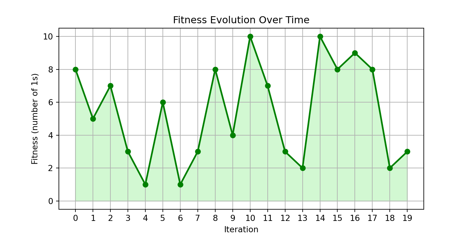
#### Example of a fitness plot with new summed fitness scoreiterations =20fitness_over_time = np.random.randint(0, n +1, size=iterations)# Line plot of fitness over iterationsplt.figure(figsize=(8, 4))plt.plot(range(iterations), fitness_over_time, marker='o', color='green', linestyle='-', linewidth=2)plt.fill_between(range(iterations), fitness_over_time, color='lightgreen', alpha=0.4)plt.title(f"Fitness Evolution Over Time")plt.xlabel("Iteration")plt.ylabel("Fitness (number of 1s)")plt.xticks(np.arange(0, iterations, step=1)) # The step shows whole numbers on the x-axis
([<matplotlib.axis.XTick object at 0x00000215F3A05FD0>, <matplotlib.axis.XTick object at 0x00000215D1301D10>, <matplotlib.axis.XTick object at 0x00000215F3A45BD0>, <matplotlib.axis.XTick object at 0x00000215F3A46350>, <matplotlib.axis.XTick object at 0x00000215F3A46AD0>, <matplotlib.axis.XTick object at 0x00000215F3A47250>, <matplotlib.axis.XTick object at 0x00000215F3A479D0>, <matplotlib.axis.XTick object at 0x00000215F3AA4190>, <matplotlib.axis.XTick object at 0x00000215F3AA4910>, <matplotlib.axis.XTick object at 0x00000215F3AA5090>, <matplotlib.axis.XTick object at 0x00000215F3AA5810>, <matplotlib.axis.XTick object at 0x00000215F3AA5F90>, <matplotlib.axis.XTick object at 0x00000215F3AA6710>, <matplotlib.axis.XTick object at 0x00000215F3AA6E90>, <matplotlib.axis.XTick object at 0x00000215F3AA7610>, <matplotlib.axis.XTick object at 0x00000215F3AA7D90>, <matplotlib.axis.XTick object at 0x00000215F3AC4550>, <matplotlib.axis.XTick object at 0x00000215F3AC4CD0>, <matplotlib.axis.XTick object at 0x00000215F3AC5450>, <matplotlib.axis.XTick object at 0x00000215F3AC5BD0>], [Text(0, 0, '0'), Text(1, 0, '1'), Text(2, 0, '2'), Text(3, 0, '3'), Text(4, 0, '4'), Text(5, 0, '5'), Text(6, 0, '6'), Text(7, 0, '7'), Text(8, 0, '8'), Text(9, 0, '9'), Text(10, 0, '10'), Text(11, 0, '11'), Text(12, 0, '12'), Text(13, 0, '13'), Text(14, 0, '14'), Text(15, 0, '15'), Text(16, 0, '16'), Text(17, 0, '17'), Text(18, 0, '18'), Text(19, 0, '19')])
plt.grid(True)plt.show()
The plot above tracks how fitness improves or changes across iterations in an optimization algorithm, giving insight into the convergence of the algorithm.
Comparing OneMax Problem to Greedy Algorithm
If a greedy search algorithm is used and is allowed to randomly add one to or subtract one from the current solution \(s\) to create the next possible solution \(v\) for solving the one-max problem, that is, it is allowed to move one and only one step to either the left or the right of the current solution in the landscape of the solution space.
Without knowledge of the landscape of the solution space, the search process will easily get stuck in the peaks of this solution space.
Hence, most researchers prefer using the one-max problem as an example because it is easy to implement and also because it can be used to prove if a new concept for a search algorithm is correct.
The Knapsack Problem is a classic NP-complete optimization problem, where you are given a set of items, each with a weight and a value.
The goal is to determine the number of each item to include in a collection so that the total weight is less than or equal to a given limit and the total value is as large as possible.
Types of Knapsack Problems:
0/1 Knapsack Problem:
Each item can be included (1) or excluded (0) in the knapsack.
You cannot break items into smaller parts. \(\max_{s \in A} f(s) = \sum_{i=1}^{n} s_i v_i, \quad \text{subject to} \quad w(s) = \sum_{i=1}^{n} s_i w_i \leq W, \quad s_i \in \{0, 1\}\) Where \(v_i\) is the value associated with \(s_1\) and \(w_i\) is the weight associated with \(s_i\)
Fractional Knapsack Problem:
You can break items into smaller parts and include fractions of them in the knapsack.
Ratio = \(\frac{v_i}{w_i}\), where \(v_i\) is the value of item \(i\), and \(w_i\) is the weight of item \(i\).
NP Complete
NP (Nondeterministic Polynomial Time): A problem is in NP if a solution can be verified in polynomial time by a deterministic algorithm. In other words, given a solution, it is possible to check if it is correct relatively quickly (in polynomial time). However, finding the solution itself might take much longer (potentially exponential time) unless the problem can also be solved in polynomial time.
NP-complete refers to a class of problems in computational complexity theory that are both NP (nondeterministic polynomial time) and every problem in NP can be reduced to it in polynomial time
NP-hard problems are optimization or decision problems that are at least as difficult to solve as the hardest problems in NP (nondeterministic polynomial time).
Unlike NP-complete problems, NP-hard problems do not have to be verifiable in polynomial time. This means that while it may be incredibly hard to find an optimal solution, even verifying a proposed solution might take more than polynomial time.
Essentially, NP-hard problems are hard to solve optimally, and their complexity often prevents efficient algorithms from finding or checking solutions within a reasonable time frame.
NP-hard problems are broader and potentially harder than NP-complete problems because they can include problems that aren’t even in NP. They may not have a polynomial-time verification process.
Key Characteristics of NP-complete Problems
Difficult to solve: No known algorithms can solve NP-complete problems efficiently (in polynomial time) for all instances.
Verification in polynomial time: If someone provides a solution, it can be verified quickly. Equivalence to other NP-complete problems: If one NP-complete problem can be solved in polynomial time, all NP-complete problems can be solved in polynomial time.
Knapsack Problem: The 0/1 knapsack problem is NP-complete. Finding the optimal solution is hard, but verifying if a solution meets the constraints and maximizes value can be done in polynomial time.
The Fractional knapsack problem is not NP-complete and can be solved in polynomial time using a greedy algorithm.
The Travelling Salesman is a NP-hard problem.
Example Fractional Knapsack Problem
Items Available: - Item 1: Value = 10, Weight = 5 kg - Item 2: Value = 40, Weight = 10 kg - Item 3: Value = 30, Weight = 15 kg
Objective: Maximize the total value without exceeding Knapsack Capacity of 15 kg.
The greedy algorithm works well by prioritizing items with the highest value-to-weight ratio.
0/1 Knapsack Problem requires more complex algorithms like dynamic programming to find the optimal solution over the Fractional Knapsack Problem
Greedy Algorithm for Fractional Knapsack
Step 1: Calculate Value-to-Weight Ratio:
Item 1: 10/5=2
Item 2: 40/10=4
Item 3: 30/15=2
Step 2: Sort Items by Ratio (Descending): Item 2, Item 1, Item 3
Step 3: Fill the Knapsack:
Take Item 2 (10 kg, Value = 40).
Take as much of Item 1 as possible (5 kg, Value = 10).
Results: Total Weight = 15 kg, Total Value = 50.
Binary to Decimal (B2D) Problem: B2D-1
The binary to decimal model is often used in optimization problems, particularly in the context of genetic algorithms and heuristic methods.
With a minor modification, the solution space of the one-max problem can be simplified as the solution space of another optimization problem.
The model uses binary strings to represent numbers. Each string represents a decimal number when interpreted in binary form.
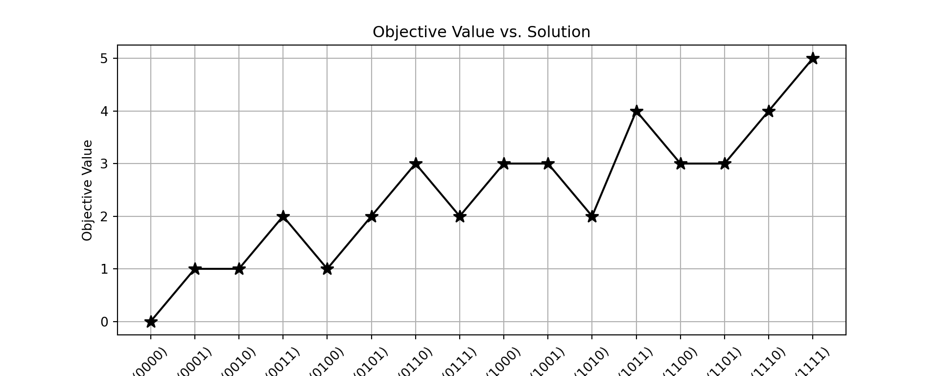
The B2D-1 problem is to maximize the value of the objective function of a binary string.
Characteristics and Visualization of B2D-1
These two examples are possible landscapes to the B2D problem.
The first chart to the left implies that there are only two possible next states (candidate solutions) that can be generated from the current solution except for solutions (0000) and (1111), which can only be moved to the right and to the left, respectively.
If another search algorithm can generate a new candidate solution by randomly inverting (flipping) one of the subsolutions of the current solution, the number of possible states of the new candidate solution will be \(n\), where \(n\) is the number of subsolutions.
OneMax
B2D with Deception: B2D-2
B2D deception problems mislead optimization algorithms away from finding the global optimum by presenting local optima that seem promising but are actually suboptimal.
Used to test whether a search algorithm is capable of escaping local optima or not.
Deception problems highlight the necessity of exploration in heuristic algorithms, such as introducing diversity through mutation or crossover in genetic algorithms. If the algorithm becomes too greedy and focuses only on local fitness improvements (exploitation), it may get stuck at deceptive local optima.
Continuous Optimization Problems
Unlike the COP, the possible solutions for a continuous optimization problem are typically “uncountably infinite.” This means that the number of solutions in the solution space is tantamount to the number of real values in the given space, that is, infinite.
Single-objective optimization problem (SOP)
The Ackley optimization problem
Multi-objective optimization problem (MOP)
The Schaffer Min-Min Global Optimization Problem
Single-objective Optimization Problem (SOP)
A single-objective optimization problem involves finding the best solution from a set of feasible solutions based on a single objective function. The goal is to either maximize or minimize this objective function.
\[\underset{s \in \mathbb{R}^n}{\text{opt}} f(s), \quad \text{subject to } \, c_i(s) \odot b_i, \quad i = 1, 2, \ldots, m,\]
where
\({R}^n\) and \({R}\) are the domain and codomain, respectively,
\(f(s) {R}^n\) and \({R}\) is the objective function to be optimized,
\(c_i(s): {R}^n\) and \({R}\odot b_i, \quad i = 1, 2, \ldots, m,\) are the constraints,
and \(opt\) and \(\odot\) are as given in Definition 1 as <, >, =, ⩽, or ⩾.
Ackley Function: A Single Optimization Problem
The Ackley Function is a widely used benchmark function for testing optimization algorithms. It is characterized by its multi-modal nature with a nearly flat outer region and a large hole at the center.
Applications
Used as a standard test case in evaluating the performance of optimization algorithms like genetic algorithms, simulated annealing, and particle swarm optimization.
Relevant in fields such as machine learning, control systems, and operations research.
Limitations
The function’s large search space and numerous local minima make it difficult for algorithms to converge to the global minimum.
Large importance of balancing exploration and exploitation in optimization strategies when dealing with the Ackley Function.
Explanation of Ackley Function(x, y)
Computes the value of the Ackley function given a point (x, y) in the search space.
The optimization algorithm optimizes the Ackley function to find the point where it reaches its minimum. It initializes a population of random solutions, evaluates their fitness (using the Ackley function), and iteratively improves them using an optimization method (like gradient descent or a genetic algorithm).
The best solution and corresponding function value (score) are returned as the result.
Ackley function and B2D: Converting to Decimal
The Ackley function uses the binary representation, where the binary strings need to be converted to decimal values (i.e., real numbers). In this case, the converted decimal values correspond to points in the continuous search space.
For example, a binary string like 1010 can be converted into a decimal value, which can then be used as input to the Ackley function. Binary String: 1010, where the binary number is 1010_2.
Each position in the binary number represents a power of 2, starting from the right (least significant bit):
The rightmost bit (0) is \(2^0\),The next bit (1) is \(2^1\) ,The next bit (0) is \(2^2\),The leftmost bit (1) is \(2^3\).
\(1010_2= 0 ∗ 2^0+ 1 ∗ 2^1 +0 ∗ 2^2+1 ∗ 2^3\)\(= 0 ∗ 1+ 1 ∗ 2 + 0 ∗ 4 + 1 ∗ 8\)\(= 0 + 2 + 0 + 8 = 10\) Thus, the decimal equivalent of the binary string “1010” is 10. Use this value as input for the Ackley function.
Characteristics and Visualization of Ackley Function
The Ackley function is evaluated in the hypercube.
The global optimum (minimum) of the Ackley function is 𝑓(𝑠^∗)=0 is located at \(s^*=(0,0,…0)\).
This function has many local optima, which makes it hard for the search algorithm to find the global optimum.
The below example uses a random function to pull a point that we want to hit the local minima. You can imagine, this might not be the best way to do this.
PSEUDOCODE FUNCTION Ackley(s): SET a = 20, b = 0.2, c = 2 * pi SET n = length of s COMPUTE sum_sq_term = sum of squares of all elements in s COMPUTE cos_term = sum of cos(2 * pi * each element in s)
COMPUTE term1 = -a * exp(-b * sqrt(sum_sq_term / n))
COMPUTE term2 = -exp(cos_term / n)

RETURN term1 + term2 + a + e
Main Execution
SET n = 2 # Dimension of the Ackley function
Generate random vector s with elements between -30 and 30
SET s = random values in range [-30, 30] of length n
Compute the Ackley function result for the vector s
SET result = Ackley(s)
PRINT vector s PRINT Ackley function result for vector s
Ackley Function Python Implementation
import numpy as npimport matplotlib.pyplot as pltfrom mpl_toolkits.mplot3d import Axes3Dnp.random.seed(5042)# Ackley function implementationdef ackley(s): a, b, c =20, 0.2, 2* np.pi n =len(s) sum_sq_term = np.sum(s**2) cos_term = np.sum(np.cos(c * s)) term1 =-a * np.exp(-b * np.sqrt(sum_sq_term / n)) term2 =-np.exp(cos_term / n)return term1 + term2 + a + np.e# Example usage: n =2# Dimension s = np.random.uniform(-30, 30, n) # Generate random s_i values in the range [-30, 30]result = ackley(s) # Evaluate the Ackley functionprint(f"Vector s: {s}")
Vector s: [12.84779359 3.16468632]
print(f"Ackley function result: {result}")
Ackley function result: 17.91745666838746
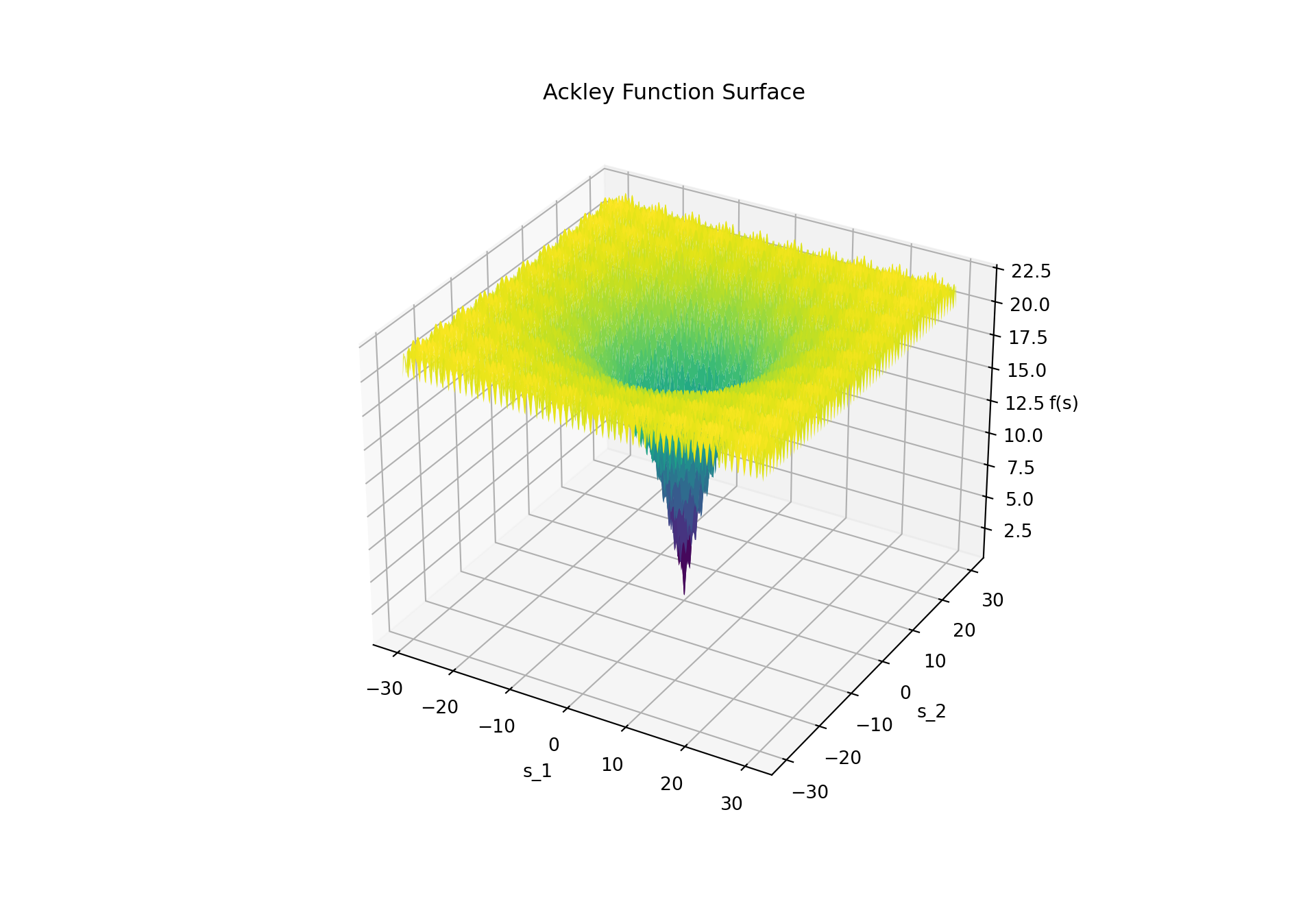
# Visualization of the Ackley functionx = np.linspace(-30, 30, 400)y = np.linspace(-30, 30, 400)X, Y = np.meshgrid(x, y)# Compute Z for the Ackley functionZ = np.array([ackley(np.array([x_val, y_val])) for x_val, y_val inzip(np.ravel(X), np.ravel(Y))])Z = Z.reshape(X.shape)# Plotting the Ackley function surfacefig = plt.figure(figsize=(10, 7))ax = fig.add_subplot(111, projection='3d')ax.plot_surface(X, Y, Z, cmap='viridis', edgecolor='none')# Customize the plotax.set_title("Ackley Function Surface")ax.set_xlabel("s_1")ax.set_ylabel("s_2")ax.set_zlabel("f(s)")# Show the plotplt.show()
Example results: Vector s: [12.8 3.16]; Ackley function result: 17.9. These results are random, so it may vary from what you see in the plot.
Distance from the Origin: The Ackley function reaches its global minimum of 0 at the origin (i.e., when both \(x_1\) and \(x_2\) are close to 0). Our vector values are quite far from the origin, which is why the function result is positive and relatively large at 17.9”
The Ackley landscape has an exponentially increasing structure as you move away from the global minimum. It has many local minima, which makes optimization algorithms prone to getting stuck in suboptimal solutions. A result like 17.9 is far from zero, and indicates that the vector is located in such a suboptimal region of the function space.
Thus, the Ackley result of 17.9 suggests that the point [12.8 3.16]; is not close to the global minimum (which is zero at the origin) and is located in a region of higher function values.
Differential Evolution with the Ackley Function
To demonstrate how an algorithm does well on the Ackley function, we can use a global optimization algorithm such as Differential Evolution, which is effective for non-convex functions with many local minima.
Differential Evolution is a population-based optimization algorithm used for solving complex multidimensional problems. It belongs to the family of evolutionary algorithms, where a population of candidate solutions evolves over time to find the global optimum of a function.
The differential_evolution function from the scipy.optimize module is a powerful optimization tool designed to solve global optimization problems. It is a type of evolutionary algorithm, which is used when the function to optimize is non-linear, has many local minima, or is not differentiable.
import numpy as npfrom scipy.optimize import differential_evolutionimport matplotlib.pyplot as pltnp.random.seed(5042)# Define the Ackley function# Ackley function implementationdef ackley(s): a, b, c =20, 0.2, 2* np.pi n =len(s) sum_sq_term = np.sum(s**2) cos_term = np.sum(np.cos(c * s)) term1 =-a * np.exp(-b * np.sqrt(sum_sq_term / n)) term2 =-np.exp(cos_term / n)return term1 + term2 + a + np.e# Set the bounds for the variables bounds = [(-30, 30), (-30, 30)]# Use differential evolution to minimize the Ackley functionresult = differential_evolution(ackley, bounds, seed=42)# Print the resultprint(f'Optimized parameters (x1, x2): {result.x}')
Optimized parameters (x1, x2): [0. 0.]
print(f'Function value at minimum: {result.fun}')
Function value at minimum: 4.440892098500626e-16
# Visualization of the Ackley functionx = np.linspace(-30, 30, 400)y = np.linspace(-30, 30, 400)X, Y = np.meshgrid(x, y)# Compute Z for the Ackley functionZ = np.array([ackley(np.array([x_val, y_val])) for x_val, y_val inzip(np.ravel(X), np.ravel(Y))])Z = Z.reshape(X.shape)# Plotting the Ackley function surfacefig = plt.figure(figsize=(10, 7))ax = fig.add_subplot(111, projection='3d')ax.plot_surface(X, Y, Z, cmap='viridis', edgecolor='none')# Customize the plotax.set_title("Ackley Function Surface (2D)")ax.set_xlabel("s_1")ax.set_ylabel("s_2")ax.set_zlabel("f(s)")# Show the plotplt.show()
Using a great function that is designed to solve problems with multiple local minimums, you can see that we got extremely close to the local minimum 0.
Multi-objective Optimization Problem (MOP)
Given a set of functions and a set of constraints, the MOP is to find the optimal value or a set of optimal values (also called Pareto front), subject to the constraints, out of all possible solutions of these functions.
The Pareto front consists of solutions where no objective can be improved without worsening at least one other objective. For example, In product design, you might want to minimize cost while maximizing performance. These two objectives are often in conflict, meaning improving one leads to trade-offs in the other.
\({R}^n\) and \({R}\) are the domain and codomain, respectively,
\(f(s) {R}^n\) and \({R}\) is the objective function to be optimized,
\(c_i(s): {R}^n\) and \({R}\odot b_i, \quad i = 1, 2, \ldots, m,\) are the constraints,
and \(opt\) and \(\odot\) are as given in Definition 1 as <, >, =, ⩽, or ⩾.
The Schaffer min-min Multi-objective Optimization Problem
The Schaffer min-min problem is a well-known test function in the field of multi-objective optimization.
It is often used to evaluate optimization algorithms due to its simplicity and well-defined structure. The problem is particularly famous for having a simple Pareto-optimal front.
The Schaffer function can be defined as a two-objective optimization problem, where the objectives are functions of a single variable x.
The goal is to minimize both of these objective functions simultaneously.
Characteristics and Visualization
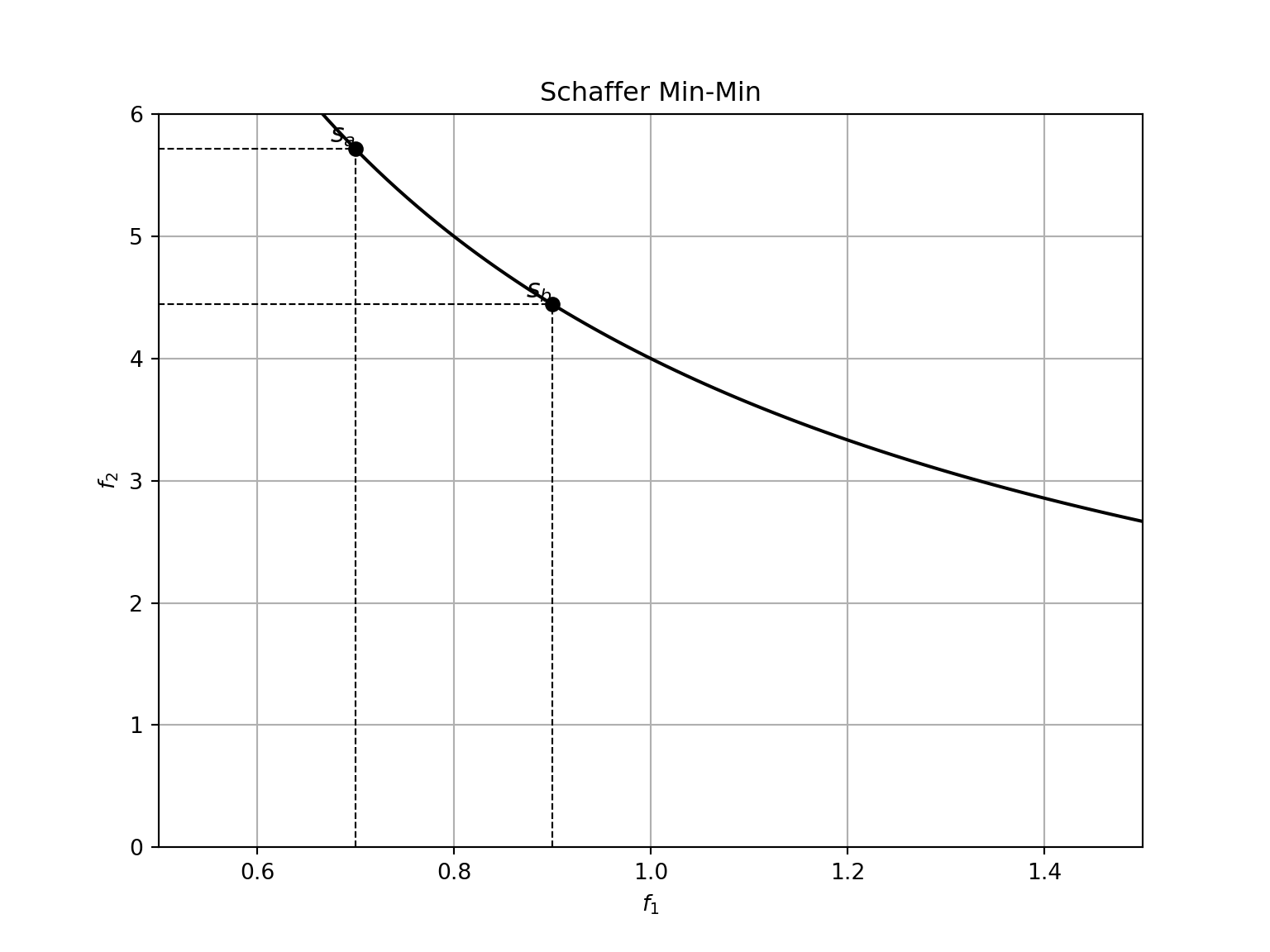
Convexity: The Pareto front of the Schaffer min-min problem is convex, making it relatively easy to identify the trade-off surface between the two objectives.
Graphically, the Pareto front of the Schaffer min-min problem can be visualized as a curve in the objective space, where \(f_1(x)\) is plotted against \(f_2(x)\) and the curve represents the set of optimal trade-offs between the two objectives.
(0.5, 1.5)
(0.0, 6.0)
scipy.optimize import minimize
minimize is a general-purpose function from scipy.optimize used for finding the minimum of a scalar function.
Uses the BFGS (Broyden–Fletcher–Goldfarb–Shanno) algorithm when no specific method is provided. This method is a quasi-Newton optimization algorithm, particularly useful for smooth unconstrained problems.
It can handle different types of optimization problems, including: Unconstrained minimization
Constrained minimization (equality and inequality constraints) Bounded minimization (where variables are limited to a certain range)
Basic Workflow:
Define the objective function (the function to minimize). Choose an initial guess for the variables.
Run the minimize function with the desired method.
Analyze the results: returns optimized variables, the function value, and other diagnostic information.
Step 1: Set up the bounds for the solution (s ∈ [-1000, 1000])
SET bounds = [-1000, 1000]
Step 2: Initialize a starting guess for the solution
SET initial_guess = 0
Step 3: Minimize the combined objective function using an optimization algorithm
CALL minimize function with combined_objective, initial_guess, and bounds STORE the result in result
Step 4: Print the optimization result
PRINT “Optimal value of s:”, result.x PRINT “f1(s):”, f1(result.x) PRINT “f2(s):”, f2(result.x) PRINT “Combined objective:”, combined_objective(result.x)
Step 5: Visualization - Create a range of values for s from -1000 to 1000
Schaffer Min-Min Python Implementation
Population Initialization: A population of random solutions is initialized within the bounds [−1000,1000]. Objective Function Evaluation: For each solution, both objective functions are evaluated.
Score Combination: The results of the two functions are combined into a single score, which can be minimized. In this case, the combination is a simple sum of f1 and f2.
Optimization Loop: Iteratively updates the solutions to find the minimum combined score using an optimization technique (e.g., gradient descent, genetic algorithm).
The plot uses the weighted sum minimization, w1 * f1(s) + w2 * f2(s) instead of plotting the Pareto front. The plot prints The optimal \(s\) value and the corresponding function values \(f1(s)\) and \(f2(s)\) at that point. The minimum combined objective function value.
import numpy as npfrom scipy.optimize import minimizeimport matplotlib.pyplot as plt# Define the two objective functions for the Schaffer problemdef f1(s):return s**2def f2(s):return (s -2)**2# Combined objective function: weighted sum of f1 and f2# You can adjust the weights to explore different trade-offs between the two objectivesdef combined_objective(s, w1=0.5, w2=0.5):return w1 * f1(s) + w2 * f2(s)# Bounds for the solution (s ∈ [-1000, 1000])bounds = [(-1000, 1000)]# Initial guess for the solutioninitial_guess = np.array([0])# Use scipy's minimize function to find the solutionresult = minimize(combined_objective, initial_guess, bounds=bounds)# Print the resultprint("Optimal value of s:", result.x[0])
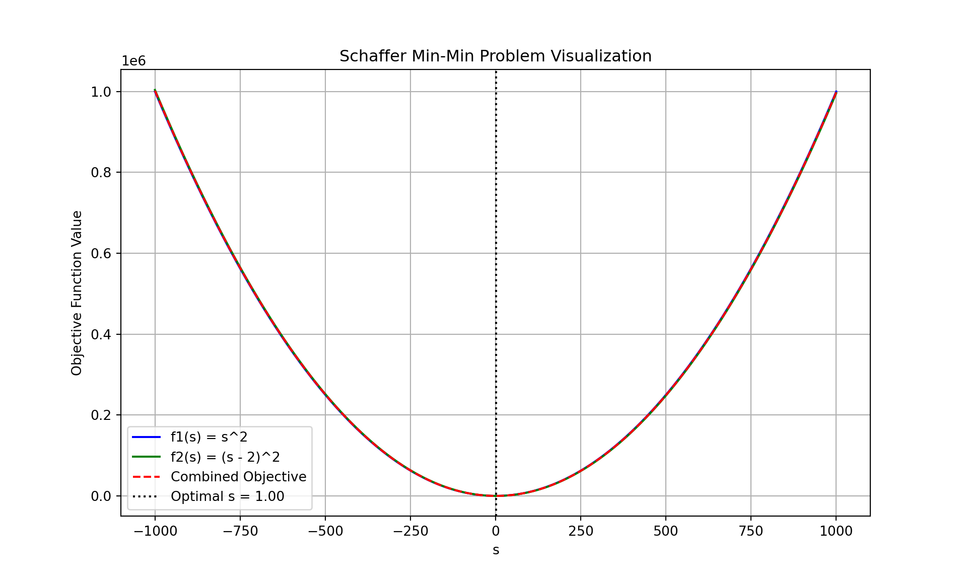
# Visualization of the objective functions and combined objectives_values = np.linspace(-1000, 1000, 400)f1_values = f1(s_values)f2_values = f2(s_values)combined_values = combined_objective(s_values)# Plottingplt.figure(figsize=(10, 6))# Plot f1(s), f2(s), and combined objectiveplt.plot(s_values, f1_values, label="f1(s) = s^2", color='blue')plt.plot(s_values, f2_values, label="f2(s) = (s - 2)^2", color='green')plt.plot(s_values, combined_values, label="Combined Objective", color='red', linestyle='--')# Mark the optimal solution foundplt.axvline(x=result.x[0], color='black', linestyle=':', label=f"Optimal s = {result.x[0]:.2f}")# Customize the plotplt.title("Schaffer Min-Min Problem Visualization")plt.xlabel("s")plt.ylabel("Objective Function Value")plt.legend()plt.grid(True)# Show the plotplt.show()
Looking at the results
The results you achieved for the Schaffer Min-Min problem look excellent, as they closely approximate the optimal solution.
Optimal value of \(s\) we found is nearly exactly \(1\), the known optimal solution for the Schaffer function.
Objective function values: \(f_1(s) = s^2 = 1.000000027\)
: \(f_2(s) = (s-2)^2 = 0.999999973\)
These values are very close to 1 for both \(f_1\) and \(f_2\), indicating that the function values at this \(s\) are near-optimal.
Combined objective: The combined objective (likely calculated as a weighted sum or some other combination of \(f_1\) and \(f_2\) is 1.00000, which is extremely close to the expected combined optimal value of 1. This negligible difference suggests that the optimization algorithm has performed very well.
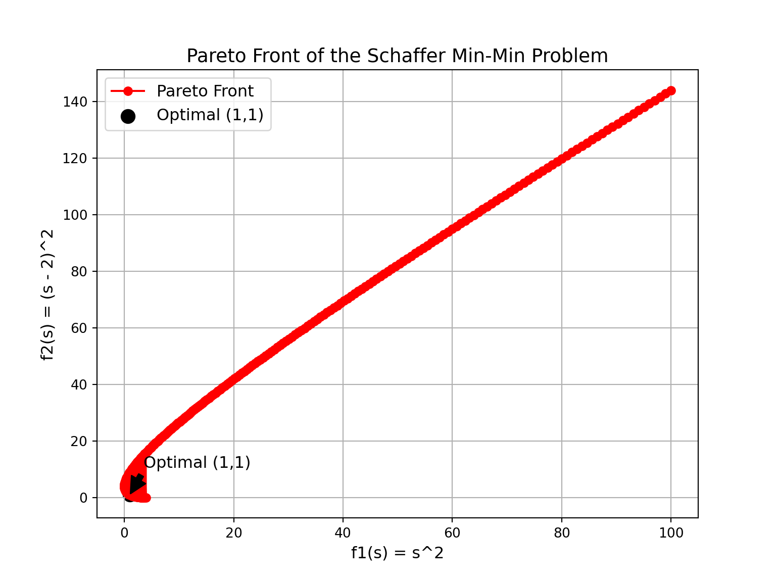
Here is the code used to generate the Pareto Front for the Schaffer Min-Min problem, filtering out only the non-dominated solutions and plotting the trade-off curve. This allows us to see \(f_1\) and \(f_2\) on the x and y axis.
There are so many ways to graph this, but the multiple dimensions makes it more difficult to see. Explore some options using generative AI.
# Generate s valuess_values = np.linspace(-10, 10, 400)# Identifying the non-dominated solutions (Pareto front)pareto_f1 = []pareto_f2 = []for s in s_values: f1_val = f1(s) f2_val = f2(s)# A point (f1, f2) is Pareto-optimal if no other point dominates itifnotany(other_f1 <= f1_val and other_f2 <= f2_val for other_f1, other_f2 inzip(pareto_f1, pareto_f2)): pareto_f1.append(f1_val) pareto_f2.append(f2_val)# Sorting to ensure a smooth Pareto front curvepareto_f1, pareto_f2 =zip(*sorted(zip(pareto_f1, pareto_f2)))# Plotting the Pareto front with a more visible optimal pointplt.figure(figsize=(8, 6))plt.plot(pareto_f1, pareto_f2, marker='o', linestyle='-', color='red', label="Pareto Front")# Mark the optimal solution (1,1) with a larger marker and annotationplt.scatter(1, 1, color='black', marker='o', s=100, label="Optimal (1,1)")plt.annotate("Optimal (1,1)", xy=(1, 1), xytext=(10, 20), textcoords="offset points", fontsize=12, color='black', arrowprops=dict(facecolor='black', shrink=0.05))# Customize the plotplt.title("Pareto Front of the Schaffer Min-Min Problem", fontsize=14)plt.xlabel("f1(s) = s^2", fontsize=12)plt.ylabel("f2(s) = (s - 2)^2", fontsize=12)plt.legend(fontsize=12)plt.grid(True)# Show the plotplt.show()
Using AI
Use the following prompt on a generative AI, like chatGPT, to learn more about the topics covered. ** evaluating optimization algorithms? Provide examples of their use in different domains.
Benchmark Problems Overview: What are benchmark problems, and why are they essential in evaluating optimization algorithms? Provide examples of their use in different domains.
Comparing Problems: Compare the OneMax problem, the Knapsack problem, and the Ackley function. Discuss the type of optimization each addresses and the challenges it presents.
Fitness Function: Write a Python function to evaluate the fitness of a binary string in the OneMax problem. Explain how this function helps in evolutionary algorithms.
Applications: Discuss real-world applications of the Knapsack problem. How do its constraints reflect practical optimization challenges?
Function Analysis: Explain why the Ackley function is challenging for optimization algorithms. What characteristics make it a good benchmark for multi-modal optimization?
Python Implementation: Use the provided Ackley function implementation to evaluate random points in the search space. Visualize the function in 3D and identify the global minimum.
Schaffer Min-Min Problem: Solve the Schaffer Min-Min problem using a weighted sum approach. Experiment with different weight combinations and discuss how they affect the solution.
Conclusions
We introduced a set of popular optimization benchmark problems, widely used to evaluate the performance of various algorithms across different types of optimization challenges. These benchmarks include the OneMax Problem, which is commonly used in evolutionary algorithm research to assess an algorithm’s capacity to evolve a binary string towards an optimal solution, specifically a string composed entirely of 1s. This problem is straightforward and serves as a foundation for evaluating basic evolutionary or heuristic methods. The Knapsack Problem is a classic combinatorial, NP-complete problem that tests algorithms’ abilities to maximize the total value of selected items without exceeding a weight limit. This problem is pivotal in assessing algorithms designed for discrete optimization tasks, where finding an optimal solution is computationally intensive.
The Ackley Function represents a single continuous optimization benchmark with a highly multi-modal landscape. It is challenging due to its numerous local minima, making it ideal for testing an algorithm’s ability to balance exploration and exploitation in continuous search spaces. In multi-objective optimization, the Schaffer Min-Min Problem serves as a benchmark, presenting a simple yet effective test for algorithms to identify Pareto-optimal solutions, as it requires the simultaneous minimization of two objectives. Collectively, these benchmark problems allow researchers and practitioners to compare the strengths and limitations of optimization algorithms across both discrete and continuous scenarios.