Python for Heuristics & NumPy

Coding Know-How

• In the field of heuristic modeling, coding know-how is not just a tool—it’s an essential skill that enables you to experiment, adapt, and optimize solutions for complex, real-world problems. As we explore heuristic methods in this MSBA course, having a strong foundation in coding, especially in Python, will allow you to implement and test algorithms efficiently.
• Good coding practices, such as writing clear, modular code and incorporating meaningful comments, are critical for both readability and collaboration. By starting with simple Python examples that highlight these principles, we’ll build the groundwork for more sophisticated modeling tasks, from randomization techniques to optimization algorithms, equipping you with both technical skills and best practices for professional code development.

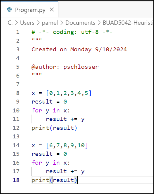
What problems does this code have?

• Multiple instantiations of the same code within a program cause problems + More opportunities for errors
  • More maintenance
• Blocks of reusable code solve this problem
  • These are called functions
• To avoid resetting the value of result and preserve the sum of both lists, you can accumulate the sums in a single loop or retain the value of result between the loops.
• Alternatively, you can use Python’s built-in sum() function to simplify the code like below.

x1 = [0, 1, 2, 3, 4, 5]
x2 = [6, 7, 8, 9, 10]

print(sum(x1))
print(sum(x2))

15
40

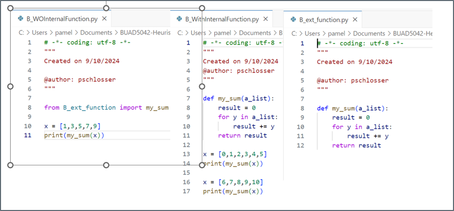
Writing Programs with Internal Functions

• Indentation: Function statements must be indented.
• Arguments: Variables passed from calling program to the function
  • a_list is an argument required by my_sum
    
  • a_list assumes value of x passed from main
• Return: a return statement sends variables back to main program
  
• Variable scope: where execution begins
  • The first un-indented line that is not a function definition or a global variable
  • a_list is defined only in the function when it runs
• Place all functions above the “main” program
  • Must be defined before they are used

def my_sum(a_list):
    result = 0
    for y in a_list:
        result += y
    return result
    
x = [0,1,2,3,4,5]
print(my_sum(x))

15

Understanding The Loop

for y in a_list:
   result += y
return result

• A loop is a way to repeat the same action for every item in a collection (like a list).
• For y in a_list means, take each item in a_list one at a time, and call it y.
  • For example, if a_list is [0, 1, 2, 3, 4, 5], the loop will do the following:
  • First loop: set y = 0, result = 0 + 0 (result is now 0).
  • Second loop: Then, set y = 1, result = 0 + 1 (result is now 1).
  • Third loop: then y = 2, result = 1 + 2 (result is now 3). and so on, until all the numbers in the list have been used.

program.py

Procedural Programming vs Object Oriented Programming (OOP)

• Procedural Programming:
  • In Python, you can program .py files where the code is organized into functions, with data often being passed around between them.
  • Functions perform specific tasks but do not group behavior and state (data) together.
  • All the code tends to be written in one or a few large files, without much encapsulation or separation of concerns.
  • The textbook uses OOP, I will supplement with procedural models.
• OOP:
  • In Python, you can use OOP to separate different parts of your code, such as algorithms, test cases, and libraries, by encapsulating them in different classes or modules. This leads to a more organized and maintainable codebase.
  • What can you separate:
    • Algorithm (Core Logic): You encapsulate the algorithm or formula into a class or function within a class.
    • Library (Utility Functions):Any utility functions or reusable logic can be put into a separate class (or module) that handles common operations.
    • Test Cases (Validation):Testing is often done through separate classes or functions, typically in a separate module.
• Both are fine ways to program, but note that both approaches differ in regards to solving problems in Python. Procedural programming focuses on structuring code into functions and sequences of instructions, making it straightforward and ideal for simpler tasks or smaller projects. In contrast, OOP organizes code around objects, which encapsulate data and behavior, allowing for greater modularity, reuse, and scalability.
• While procedural programming excels in scenarios where tasks are linear, OOP excels in complex applications that benefit from abstraction and inheritance. Python supports both paradigms, letting developers choose the best approach based on the problem’s complexity and design requirements.

Libraries to Note

libraries.py

Numpy Basics

• NumPy stands for numerical Python, suggesting that it targets scenarios that are numerically demanding. The base Python interpreter tries to be as general as possible in many areas, which often leads to quite a bit of overhead at run-time.
• NumPy uses specialization for numerical components as its major approach to avoid overhead and to be as good and as fast as possible in certain application scenarios.
• Vectorization is a powerful concept for writing concise, easy-to-read, and easy-to-maintain code in fields such as finance and algorithmic trading. With NumPy, vectorized code does not only make code more concise, but it also can speed up code execution considerably (by a factor of about eight in the Monte Carlo simulation, for example).

import numpy as np

Basic Array Creation

• The np.array function in NumPy is used to create an array (a grid of values) from data provided as lists, tuples, or other array-like structures. The resulting NumPy array is a powerful and flexible structure for mathematical operations, as it supports multiple dimensions, broadcasting, and various data types.

# Creating a simple numpy array from a Python list
array = np.array([1, 2, 3, 4])
print("Array:", array)

Array: [1 2 3 4]

• np.arange() is a NumPy function that generates an array with evenly spaced values within a given range.

array = np.arange(1, 5)  # Generates [1, 2, 3, 4]
print("Array:", array)

Array: [1 2 3 4]

Element-Wise Operations

• Element-wise operators are mathematical or logical operations applied independently to corresponding elements in arrays or matrices of the same shape.
• Each element in one array is combined with the corresponding element in the other array using the operator.
• In the context of arrays (such as in NumPy), common element-wise operators include basic arithmetic operators:
  • Element-wise addition +
  • Element-wise subtraction -
  • Element-wise multiplication *
  • Element-wise division /
  • Element-wise exponentiation **

# Performing element-wise addition
array = np.array([1, 2, 3, 4])
added_array = array + 5
print("Added Array:", added_array)

Added Array: [6 7 8 9]

a = np.array([1, 2, 3])
b = np.array([4, 5, 6])
c = a + b
print(c)

[5 7 9]

Taking an Exponent: np.exp

• np.exp is a function in the NumPy library that calculates the exponential of all elements in an input array. Specifically, it computes the base-e exponential function, which is 𝑒^𝑥, where 𝑒 is Euler’s number (approximately 2.71828), and 𝑥 is the input array or scalar.

# Applying np.exp to the array
array = np.array([1, 2, 3, 4])
exp_array = np.exp(array)
print("Exponential Array:", exp_array)

Exponential Array: [ 2.71828183  7.3890561  20.08553692 54.59815003]

• np.exp from Simulated Annealing example
• This function is part of a Simulated Annealing algorithm, specifically handling the temperature decay mechanism to decide whether to accept a new solution, even if it’s worse than the current one. Here’s a breakdown of the function based on the np.exp command and the logic:
  • tmp_obj_val: The objective value of a new (temporary) solution.
  • obj_val: The objective value of the current solution. temperature: The current temperature in the simulated annealing process, which controls how likely the algorithm is to accept worse solutions.
  • A random number r between 0 and 1 is generated. This represents a threshold for whether the new solution will be accepted using random.rand()
  • The probability p of accepting the new solution is computed using the exponential function.
  • If the random value r is less than the calculated probability p, the function returns True, meaning the new solution is accepted (even if it’s worse). If r is greater than p, the new solution is rejected, and the current solution is maintained.
• The function decides whether to accept a new solution in simulated annealing, balancing exploration and exploitation based on the temperature and objective values of the solutions. The np.exp() function ensures that worse solutions have a chance to be accepted, particularly early in the process, fostering a broader search space.

# Simulated annealing temperature decay
def determine(self, tmp_obj_val, obj_val, temperature):
     r = np.random.rand()
     p = np.exp((tmp_obj_val - obj_val) / temperature)
     return r < p

Taking a square root: np.sqrt()

• np.sqrt is a function in NumPy that returns the non-negative square root of an element-wise input array. It operates on each element of the array and computes the square root.

# Applying np.sqrt to the array
sqrt_array = np.sqrt(array)
print("Square Root Array:", sqrt_array)

Square Root Array: [1.         1.41421356 1.73205081 2.        ]

• The Ackley function is commonly used as a benchmark problem in optimization, and is known for its many local minima. The Ackley function uses the np.sqrt within its formula.

def ackley(s):
     a, b, c = 20, 0.2, 2 * np.pi
     n = len(s)
     sum_sq_term = np.sum(s**2)
     cos_term = np.sum(np.cos(c * s))
     term1 = -a * np.exp(-b * np.sqrt(sum_sq_term / n))
     term2 = -np.exp(cos_term / n)
     return term1 + term2 + a + np.e

Random Number Generation

• The np.random.rand function in NumPy generates random floating-point numbers from a uniform distribution between 0 (inclusive) and 1 (exclusive), meaning the generated numbers will always include 0 (inclusive) but never reach 1 (exclusive).
• Random numbers are key to both genetic algorithms (mutation, crossover) and simulated annealing (random perturbations).
• The example below selects uses np.random.rand() to generate 5 uniform random numbers between 0 and 1 [0,1). It is saved in a variable rand_nums and the values in the variable are printed.

rand_nums = np.random.rand(5)
print(rand_nums)

[0.42258775 0.41449356 0.83578836 0.24556806 0.63062298]

Standard Normal Distribution

• The np.random.standard_normal function in NumPy generates random floating-point numbers from a standard normal (Gaussian) distribution, with a mean of 0 and a standard deviation of 1.
• Generating 5 random numbers from a standard normal distribution (mean=0, std=1).

# Generating random values from the standard normal distribution
random_values = np.random.standard_normal(5)
print("Random Standard Normal Values:", random_values)

Random Standard Normal Values: [ 0.21722573  0.08161093  0.0738901   0.70165888 -0.11269229]

np.random.uniform

The np.random.uniform function in NumPy is used to generate random floating-point numbers drawn from a uniform distribution over a specified range. For example, in hill climbing, the algorithm often starts with a random solution that can be simulated with np.random.uniform.

# Generate a random starting point for the hill climbing algorithm
random_start = np.random.uniform(low=-10, high=10, size=5)
print(f"Random start: {random_start}")

Random start: [ 7.60625241 -4.77577367 -5.90068767 -8.78667658 -6.55427277]

np.random.randint

• The np.random.randint function in NumPy is used to generate random integers within a specified range.

• np.random.randint(low, high=None, size=None, dtype=int)

  • low: The lower boundary of the random integers (inclusive).
  • high: The upper boundary of the random integers (exclusive). If not provided, random integers are generated between 0 and low.
  • size: The shape of the output array (optional). If not provided, a single integer is returned.
  • dtype: The desired data type of the output array, by default int.

# Generate 5 random integers between 10 and 20
random_integers = np.random.randint(10, 20, size=5)
print(random_integers)

[10 12 16 15 13]

• We can use np.random.randint to generate a 2D array instead of a 1D array by specifying the size parameter as a tuple that indicates the shape of the array.

random_2d_array = np.random.randint(10, 20, size=(3, 5)) 
print(random_2d_array)

[[19 14 19 13 19]
 [15 15 17 18 13]
 [18 15 19 17 14]]

np.random.randint from Simulated Annealing

• This function, transit(), is used to modify a solution sol as part of a heuristic search process, likely for algorithms like genetic algorithms, hill climbing, or simulated annealing. The goal is to explore the solution space by introducing a small, random change (or “transition”) to the current solution.

  • The function takes a single argument, sol, which is likely a binary array or list (a list of 0s and 1s).
  • t = sol.copy(): A copy of the solution sol is made, named t. This is important because we don’t want to modify the original solution directly; instead, we work on the copy t.
  • i = np.random.randint(len(sol)): The randint function from NumPy is used to randomly select an index i between 0 and the length of sol - 1. This selects a random position in the solution array.
  • t[i] ^= 1: This is a bitwise XOR operation. In the context of a binary solution (a list of 0s and 1s), it flips the value at index i:If t[i] is 0, it becomes 1.If t[i] is 1, it becomes 0. This operation introduces a small, random change to the solution by flipping one bit.
  • return t: After flipping one bit, the modified solution t is returned.

  # Transition function (T)
  def transit(sol):
      new_sol = sol.copy()
      index = np.random.randint(len(sol))
      new_sol[index] = 1 - new_sol[index]  # Flip a random bit
      return new_sol

• To compare:

  • np.random.standard_normal = normal distribution with mean and sd
  • np.random.rand = uniform distribution between [0,1)
  • np.random.uniform = uniform over a specified range
  • np.random.randint = random integers within a specified range

Sorting the data: np.argsort

• The np.argsort function in NumPy returns the indices that would sort an array along a specified axis. This allows you to reorder elements based on their sorted order without actually changing the original array.

• In various evolutionary algorithms (such as genetic algorithms or simulated annealing), selecting the most “fit” or optimal solutions from a population is crucial for convergence toward the global optimum.

• By sorting individuals based on fitness, the algorithm can efficiently identify the most promising candidates for further exploration (e.g., crossover, mutation) or intensify the search around high-quality solutions.

• The use of np.argsort allows for a fast, reliable way to rank individuals, ensuring that the evolutionary process focuses on refining the best candidates and discarding those with lower potential.

# Dummy population and fitness values
population = np.array([[1, 2], [3, 4], [5, 6], [7, 8], [9, 10]])

# Assign dummy fitness values
fitness = np.array([10, 30, 20, 40, 50]) 

# Sort population based on fitness
indices = np.argsort(fitness)
print(indices) 
sorted_population = population[indices]

# Select top 3 individuals
top_individuals = sorted_population[:3] 
print(top_individuals)

[0 2 1 3 4]
[[1 2]
 [5 6]
 [3 4]]

Selecting the Max: np.argmax

• The np.argmax function in NumPy returns the index of the maximum value in an array along a specified axis.
• Finding the Index of the Maximum Element in a 1D Array: The np.argmax function returns the index of the first occurrence of the maximum value in the array. In this case, the maximum value is 7, and it occurs at index 2.

arr = np.array([1, 3, 7, 2, 5])
index = np.argmax(arr)
print("Array:", arr)
print("Index of max element:", index)
print("Max element:", arr[index])

Array: [1 3 7 2 5]
Index of max element: 2
Max element: 7

Array: [1 3 7 2 5]

• Using np.argmax with a 2D Array (Row-wise & Column-wise): np.argmax can work on multi-dimensional arrays. By specifying axis=0 or axis=1, you can find the maximum values column-wise or row-wise, respectively. For axis=0, you get the indices of the maximum elements for each column, and for axis=1, you get them for each row.

arr_2d = np.array([[1, 2, 3], [4, 5, 1], [0, 6, 2]])

# Find the index of the max element in the flattened array
max_index_flat = np.argmax(arr_2d)
print("Flattened array index:", max_index_flat)

Flattened array index: 7

• Number 6 is in index 7, starting at index 0 and counting up across each row.
  [[1 2 3]
  [4 5 1]
  [0 6 2]]

# Find the index of the max element along each column (axis=0)
max_index_col = np.argmax(arr_2d, axis=0)
print("Max element index for each column:", max_index_col)

Max element index for each column: [1 2 0]

• 4 is in index 1, 6 is in index 2, and 3 is in index 0, counting across each column starting at index 0. [[1 2 3]
  [4 5 1]
  [0 6 2]]

# Find the index of the max element along each row (axis=1)
max_index_row = np.argmax(arr_2d, axis=1)
print("Max element index for each row:", max_index_row)

Max element index for each row: [2 1 1]

• 3 is in index 2 in the row, 5 is in index 1, and 6 is in index 1, counting across each row starting at index 0. [[1 2 3]
  [4 5 1]
  [0 6 2]]

Formula vs LaTex vs Python

• A numerical method used to approximate the solution of stochastic differential equations (SDEs) like the Geometric Brownian Motion (GBM). This method discretizes the continuous time process into small time steps and approximates the evolution of the stochastic process.
• The formula is central in financial mathematics, particularly in the modeling of asset prices. This model is widely used to describe the evolution of stock prices and other financial assets over time in a stochastic (random) way. Here’s a breakdown of the components and how they fit into finance:
  • Formula: \(S_T = S_0 \exp((r - 0.5 \sigma^2) T + \sigma z \sqrt{T})\)
  • In LaTex: S_T = S_0 ((r - 0.5 ^2) T + z )
  • In Python this translates to the following: S_T = S_0 * exp((r - 0.5 * sigma ** 2) * T + sigma * z * sqrt(T))

Calculating Wall Time

• Wall time refers to the real-world time that elapses from the start to the end of a process or block of code.
• time.time(): Returns the current time in seconds since the epoch (January 1, 1970). This uses the time module. When running, save it to a start_time variable.

import time
start_time = time.time()

• Execute the block of code you want to measure and end the time.

end_time = time.time()

• Subtract the start time from the end time to get the elapsed wall time and then print the elapsed time.

elapsed_time = end_time - start_time
print(f"Wall time: {elapsed_time:.2f} seconds")

Wall time: 0.01 seconds

An Example Modelling Stock Prices

• The model simulates a Geometric Brownian Motion (GBM), a widely used stochastic process in financial mathematics to model the evolution of stock prices over time. This process assumes that stock prices follow a log-normal distribution, incorporating key parameters such as the initial stock price (S0), risk-free rate (r), time horizon (T), and volatility (sigma).
• The model calculates the potential future stock prices (ST) using a mathematical formula that combines deterministic and random components, reflecting the inherent uncertainty and growth trends in financial markets. By generating a large number of simulated outcomes, the model enables analyses such as estimating expected returns, assessing risk, and valuing options, providing valuable insights for decision-making in finance.

\(S_T = S_0 \exp\left( (r - 0.5 \sigma^2) T + \sigma Z \sqrt{T} \right)\)

• The terminal stock price \(S_T\) is modeled using the Geometric Brownian Motion (GBM), a common approach to model stock prices.
  • \(S_0\): The initial stock price.
  • \(r\): The risk-free interest rate.
  • \(T\): Time to maturity (in years).
  • \(\sigma\): The volatility of the stock.
  • \(S_T\): The terminal stock price at time \(T\).
  • \(Z\): A random variable drawn from a standard normal distribution.

Comparing Model Clock Time With/Without NumPy

• The primary difference in wall time between the two approaches stems from the computational efficiency of NumPy compared to Python’s built-in modules and loops.

Without Numpy

• a Python loop iterates 1,000,000 times, and the math.exp, random.gauss, and math.sqrt functions are called repeatedly within the loop to calculate values. This results in higher wall time due to the overhead of Python’s interpreted loop and the sequential calls to these functions.

import random
from math import exp, sqrt
import time 

# Initial stock price
S0 = 100 

# Risk-free rate
r = 0.05 

# Time horizon (1 year)
T = 1.0 

# Volatility
sigma = 0.2 

values = []  

# Start tracking wall time
start_time = time.time()

for _ in range(1000000):  
     ST = S0 * exp((r - 0.5 * sigma ** 2) * T +
        sigma * random.gauss(0, 1) * sqrt(T))  
     values.append(ST)  

# End tracking wall time
end_time = time.time()


# Calculate time difference
wall_time = end_time - start_time

# Print timing information
print(f"Wall time: {wall_time:.2f} s")

Wall time: 0.67 s

With Numpy

• In contrast, the NumPy-based implementation below leverages vectorized operations. NumPy handles the entire computation in a single step using efficient, low-level C routines optimized for performance. For example:
  • The entire random sample generation is done in one call (np.random.standard_normal(1000000)).

import numpy as np
import time 

# Initial stock price
S0 = 100 

# Risk-free rate
r = 0.05 

# Time horizon (1 year)
T = 1.0 

# Volatility
sigma = 0.2 

# Start tracking wall time
start_time = time.time()

ST = S0 * np.exp((r - 0.5 * sigma ** 2) * T +
    sigma * np.random.standard_normal(1000000) * np.sqrt(T))

# End tracking wall time
end_time = time.time()

# Calculate time difference
wall_time = end_time - start_time

# Print timing information
print(f"Wall time: {wall_time:.2f} s")

Wall time: 0.03 s

• Mathematical operations like exp and sqrt are applied to entire arrays at once. These optimizations significantly reduce the wall time, as the process avoids Python-level overhead and directly utilizes optimized native code. As a result, the NumPy implementation is typically faster, making it better suited for tasks requiring a high volume of computations.

Using AI

• Use the following prompt on a generative AI, like chatGPT, to learn more about the topics covered.
• Reusable Code: Why is using functions in Python important? Write a function to calculate the sum of a list and explain how it makes the code more maintainable.
• Internal vs External Functions: Compare internal and external function definitions in Python. Create a simple example using an external Python file for function imports.
• OOP vs Procedural Programming: Explain the differences between Object-Oriented Programming and Procedural Programming. Which approach would you choose for building a reusable library, and why?
• Array Operations: Create a NumPy array from a Python list and perform element-wise addition, subtraction, multiplication, and division. Discuss the advantages of using NumPy arrays over Python lists for such operations.
• Vectorization: Explain the concept of vectorization in NumPy. Write vectorized code to add two arrays and compare its performance to a loop-based implementation.
• Exponential Function: Using np.exp, implement a function that computes the probability of accepting a new solution in a simulated annealing algorithm. Explain how the exponential function impacts the search process.
• Square Root: Write a Python script to compute the square root of all elements in a NumPy array using np.sqrt. Discuss a practical application of this operation.
• Sorting with np.argsort: Create a NumPy array of random fitness scores. Use np.argsort to rank individuals and extract the top three scores.
• Uniform Distribution: Generate an array of random numbers between -10 and 10 using np.random.uniform. How might this be useful in optimization algorithms like hill climbing?
• Normal Distribution: Use np.random.standard_normal to generate random numbers from a normal distribution. Visualize the distribution using a histogram.