Contingency Tables and Chi-Squared

Published

August 9, 2024

The goal of this lesson is to teach you probability calculations via contingency tables. We will also conduct our first hypothesis tests, which is the chi-squared test for independence and the chi-squared test of goodness of fit.

####################################
# Project name: Computing and Interpreting Chi-Square
# Data used: stem.csv, and stemGOF from CMS
# Libraries used: N/A
####################################

At a Glance

In order to succeed in this section, you will need to learn how to create and calculate probability inside a contingency table, when we have two categorical variables, and conduct our first hypothesis test, the chi-squared test of independence.

Lesson Objectives

Compute probability regarding two categorical variables inside contingencies tables.
Calculate and interpret the chi-squared statistic for the test of independence.
Calculate and interpret the chi-squared statistic for the goodness of fit test.

Consider While Reading

In this lesson, we move from simply describing data to making inferences. We learn about contingency tables in regards to calculating probability and are able to calculate and interpret the Chi-squared statistic for the test of independence.
As you read and listen to the materials for this lesson, pay attention to the concepts, and pay attention to how those concepts are applied. There are rules for calculating and combining probabilities that are important for you to know to solve the problem sets and to solve real-life problems. Take note of the applicability of the normal distribution, which is a major cornerstone for statistical analysis.

Contingency Tables

A contingency table generally shows frequencies for two qualitative or categorical variables, x and y.
Each cell represents a mutually exclusive combination of the pair of x and y values.

Note that each cell in the contingency table represents a frequency.
- In the above table, 174 customers under the age of 35 purchased an Under Armour product.
- 54 customers at least 35 years old purchased an Under Armour product.
The contingency table may be used to calculate probabilities using relative frequency.
- First obtain the row and column totals.
- Sample size is equal to the total of the row totals or column totals. In this case, n = 600.

Probability Rules

The addition rule refers to the probability that event A or B occurs, or that at least one of these events occurs, is the following:
\[P(A \cup B) = (P(A) + P(B) - P(A \cap B)\]
The complement rule refers to the probability of the complement of an event, \(P(A^c)\) is equal to one minus the probability of the event.
\[P(A^c) = 1-P(A)\]
Conditional probability refers to the probability of an event given that another event has already occurred.
- Given two events A and B, each with a positive probability of occurring, the probability that A occurs given that B has occurred (A conditioned on B) is equals to \(P(A|B) = (P(A \cap B)/P(B)\). Similarly, the probability that B occurs given that A has occurred (B conditioned on A) is equal to \(P(B|A) = (P(B \cap A)/P(A)\).
Marginal probability refers to the probability of an event occurring \((P(A))\), it may be thought of as an unconditional probability. It is not conditioned on another event.
The joint probability rule is determined by dividing each cell frequency by the grand total. Joint probability refers to the statistical measure that calculates the likelihood of two events occurring together and at the same point in time.
\[P(A \cap B)\]
- For example, the probability that a randomly selected person is under 35 years of age and makes an Under Armour purchase is \(P(U35 \cap UA)=174/600= .29\)
For example, this Venn Diagram illustrates the sample space for events A and B.
The union of two events (\(A \cup B\)) is the event consisting of all simple events in A or B.

Venn Diagram The intersection of two events (\(A \cap B\)) consists of all simple events in both A and B.

The complement of event A (i.e., \(A^c\)) is the event consisting of all simple events in the sample space S that are not in A.

Summary Measures for a Random Variable

The Summary Measures of a Random Variable are consistent with our discussion of Probability in the last lesson. They are copied back here for ease of reference.

Expected Value

We can calculate the expected value, or value we think is going to occur based on the type of distribution.
- Expected value is also known as the population mean \(\mu\), and is the weighted average of all possible values of \(X\).
- More specifically, \(E(X)\) is the long-run average value of the random variable over infinitely many independent repetitions of an experiment.
- For a discrete random variable \(X\) with values \(x_1, x_2, x_3, ...\) that occur with probabilities \(P(X=x_i)\), the expected value of \(X\) is the probability weighted average of the values. In the case of one random variable, that means: \[E(X) = \mu = \sum{x_iP(X=x_i)} = n*p\]

Variance

Variance of a random variable is the average of the squared differences from the mean.
- For a discrete random variable \(X\) with values \(x_1, x_2, x_3, ...\) that occur with probabilities \(P(X=x_i)\), the variance is defined as: \[Var(X) = \sigma^2 = \sum{(x_i-\mu)^2*P(X=x_i)} = n*p*(1-p)\]

Standard Deviation

Standard deviation is consistently the square root of the variance. \[SD(X) = \sigma = \sqrt{\sigma^2} = \sqrt{\sum{(x_i-\mu)^2*P(X=x_i)}}= \sqrt{np*(1-p)}\]

Calculating Probability

We could calculate the statistics in this contingency table a couple of ways. First, we could manually calculate it like below.

## Calculate Totals
TotalUnder35 <- 174 + 132 + 90
TotalUnder35  ##Total under 35 age group

[1] 396

Total35up <- 54 + 72 + 78
Total35up  ## Total 35 and older

[1] 204

TotalUA <- 174 + 54
TotalUA  ## Total Under Armour

[1] 228

TotalNike <- 132 + 72
TotalNike  ## Total Nike

[1] 204

TotalAdidas <- 90 + 78
TotalAdidas  ## Total Adidas

[1] 168

Total <- 174 + 132 + 90 + 54 + 72 + 78
Total  ##Grand Total

[1] 600

Alternatively, we could make this a matrix and use the matrix command to help us calculate the answer. This gives us all the statistics with a couple of functions and allows us to interpret from there after selecting the right information from the output.

# Put observed values in a vector by row.
x <- c(174, 132, 90, 54, 72, 78)
# Turn the vector into a matrix. In this case, we had 2 rows, 3
# columns, and entered the data by row.
o <- matrix(x, 2, 3, byrow = TRUE)
o

     [,1] [,2] [,3]
[1,]  174  132   90
[2,]   54   72   78

# Next, we could add the names of the columns and rows values using
# the dimnames() command.
dimnames(o) <- list(c("Under 35", "35 and Older"), c("Under Armour", "Nike",
    "Adidas"))
o

             Under Armour Nike Adidas
Under 35              174  132     90
35 and Older           54   72     78

# We can easily calculate the total from here.
total <- sum(o)
total

[1] 600

rowsums <- margin.table(o, 1)
rowsums

    Under 35 35 and Older 
         396          204

colsums <- margin.table(o, 2)
colsums

Under Armour         Nike       Adidas 
         228          204          168

prob <- prop.table(o)
prob  # each cell represents a joint probability

             Under Armour Nike Adidas
Under 35             0.29 0.22   0.15
35 and Older         0.09 0.12   0.13

rowprob <- margin.table(prob, 1)
rowprob  #each value represents marginal probability

    Under 35 35 and Older 
        0.66         0.34

colprob <- margin.table(prob, 2)
colprob  #each value represents marginal probability

Under Armour         Nike       Adidas 
        0.38         0.34         0.28

Take note that when subsetting from the matrix we created above, the dimnames do not serve as a column or row. so the first number is in row 1, column 1. This is distinct from data.frames, which typically have the 1st column designated for the labels.

prob[1, 1]  #corresponds to the joint probability value associated with Row 1 (Under 35), Col 1 (Under Armour)

[1] 0.29

Once we do our calculations our totals, we can ask probability questions.
When looking up an answer to the question, it makes it easier to reference the tables to ensure you are subsetting correctly.

             Under Armour Nike Adidas
Under 35              174  132     90
35 and Older           54   72     78

prob

             Under Armour Nike Adidas
Under 35             0.29 0.22   0.15
35 and Older         0.09 0.12   0.13

If a person is under 35, what is the probability they will select Under Armour? \[P(UA|under35) = (P(UA \cap under35)/P(under35))\]

# This is a conditional probability question.
174/396  #or

[1] 0.4393939

0.29/0.66  #or

[1] 0.4393939

prob[1, 1]/rowprob[1]

 Under 35 
0.4393939

What is the probability of a person 35 or older randomly selecting Nike? \[P(N|older35) = (P(N \cap older35)/P(older35))\]

# This is a conditional probability question.
72/204  # or

[1] 0.3529412

0.12/0.34  # or

[1] 0.3529412

prob[2, 2]/rowprob[2]

35 and Older 
   0.3529412

If the chance the preference was the same regardless of condition, how many people would you expect to select Nike? \[Ex(Nike)\]

# This is a expected value question.
TotalNike  # or

[1] 204

colsums[2]

Nike 
 204

We can calculate summary measures based on a variable category.

# E(X) of 35 Years or older (formula n*p)
n <- total
n  #600

[1] 600

p <- rowprob[2]
p  #.34

35 and Older 
        0.34

n * p  #Or simply the frequency for the column 35 and older

35 and Older 
         204

# Var(X) (formula n*p*(1-p))
varx <- n * p * (1 - p)
varx  #134.64

35 and Older 
      134.64

# SD(X) (formula sqrt of variance)
sdx <- sqrt(varx)
sdx  #11.60345

35 and Older 
    11.60345

Larger Contingency Table

The survey question asked participants in multiple groups the following question, “How likely are you to participate in the event in the future?”
In order to answer this question, first, lets bring in some data and calculate totals.

x <- c(197, 388, 230, 103, 137, 98, 20, 18, 18, 13, 58, 45)
o <- matrix(x, 4, 3, byrow = TRUE)
o

     [,1] [,2] [,3]
[1,]  197  388  230
[2,]  103  137   98
[3,]   20   18   18
[4,]   13   58   45

dimnames(o) <- list(c("Students", "Faculty/Staff", "Alumni", "Town Residents"),
    c("Unlikely", "Moderately Likely", "Very Likely"))
o

               Unlikely Moderately Likely Very Likely
Students            197               388         230
Faculty/Staff       103               137          98
Alumni               20                18          18
Town Residents       13                58          45

total <- sum(o)
total

[1] 1325

rowsums <- margin.table(o, 1)
rowsums

      Students  Faculty/Staff         Alumni Town Residents 
           815            338             56            116

colsums <- margin.table(o, 2)
colsums

         Unlikely Moderately Likely       Very Likely 
              333               601               391

# Lets add the grand total to the colsums
colsums <- c(colsums, total)
colsums

         Unlikely Moderately Likely       Very Likely                   
              333               601               391              1325

In this example, we can bind the data together so that it is a little easier to see. Examine the final table and compare that to the figure above.

totals <- cbind(o, rowsums)
totals

               Unlikely Moderately Likely Very Likely rowsums
Students            197               388         230     815
Faculty/Staff       103               137          98     338
Alumni               20                18          18      56
Town Residents       13                58          45     116

totals <- rbind(totals, colsums)
totals

               Unlikely Moderately Likely Very Likely rowsums
Students            197               388         230     815
Faculty/Staff       103               137          98     338
Alumni               20                18          18      56
Town Residents       13                58          45     116
colsums             333               601         391    1325

Next, let’s calculate probabilities.

prob <- prop.table(o)
prob

                  Unlikely Moderately Likely Very Likely
Students       0.148679245        0.29283019  0.17358491
Faculty/Staff  0.077735849        0.10339623  0.07396226
Alumni         0.015094340        0.01358491  0.01358491
Town Residents 0.009811321        0.04377358  0.03396226

TotalRowProb <- margin.table(prob, 1)
TotalRowProb

      Students  Faculty/Staff         Alumni Town Residents 
    0.61509434     0.25509434     0.04226415     0.08754717

TotalColProb <- margin.table(prob, 2)
TotalColProb

         Unlikely Moderately Likely       Very Likely 
        0.2513208         0.4535849         0.2950943

TotalColProb <- c(TotalColProb, sum(TotalColProb))
TotalColProb

         Unlikely Moderately Likely       Very Likely                   
        0.2513208         0.4535849         0.2950943         1.0000000

In this example, we can also bind the data together so that it is a little easier to see. Again, we are trying to get our R code in the best shape to be able to select the right information to calculate probability from it.

proportions <- cbind(prob, TotalRowProb)
proportions

                  Unlikely Moderately Likely Very Likely TotalRowProb
Students       0.148679245        0.29283019  0.17358491   0.61509434
Faculty/Staff  0.077735849        0.10339623  0.07396226   0.25509434
Alumni         0.015094340        0.01358491  0.01358491   0.04226415
Town Residents 0.009811321        0.04377358  0.03396226   0.08754717

proportions <- rbind(proportions, TotalColProb)
proportions

                  Unlikely Moderately Likely Very Likely TotalRowProb
Students       0.148679245        0.29283019  0.17358491   0.61509434
Faculty/Staff  0.077735849        0.10339623  0.07396226   0.25509434
Alumni         0.015094340        0.01358491  0.01358491   0.04226415
Town Residents 0.009811321        0.04377358  0.03396226   0.08754717
TotalColProb   0.251320755        0.45358491  0.29509434   1.00000000

Now that our tables have been tabulated, we can answer some probability questions.
What proportion of Students participated in the survey?
\(P_S= 815/1325\) or \(0.61509434\)
What proportion of Faculty/Staff remarked that they were Unlikely to participate?
\(P(U|FS) = P(U \cap FS) / P(FS) = 103/338 = 0.077735849/0.25509434 = 0.3047337\)
If a person is a Town Resident, what is the probability that they will select Very Likely?
\(P(VL|TR) = P(VL \cap TR) / P(TR) = 45/116 = 0.03396226/0.08754717 = 0.387931\)
What proportion of people would you expect to select Moderately Likely?
\(P_ML = 601/1325\) or \(0.4535849\).
What is the expected number of people would you expect to select Moderately Likely? \(E(ML) = 601\).
What is the probability that a randomly selected person is a Faculty/Staff or selects Very Likely?
\(P_FS + P_VL - P_FS \cup P_VL = 0.25509434 + 0.2950943 − 0.07396226 = 0.4762264\)

# E(X) of Moderately Likely (formula n*p)
n = total
n  #1325

[1] 1325

p = TotalColProb[2]
p  #.45358

Moderately Likely 
        0.4535849

n * p  #Or simply the frequency for the column Moderately Likely

Moderately Likely 
              601

# Var(X) (formula n*p*(1-p))
varx <- n * p * (1 - p)
varx  #328.3955

Moderately Likely 
         328.3955

# SD(X) (formula sqrt of variance)
sdx <- sqrt(varx)
sdx  #18.12

Moderately Likely 
         18.12169

Chi-Squared Test for Independence

Broadly, the test for independence tests whether or not two variables whose frequencies are represented in a contingency table have statistical independence from one another.
A test of independence – also called a chi-square test of a contingency table – is used to analyze the relationship between two qualitative variables.
Broadly, this test involves summing the squared differences between observed and expected values, combining the differences into an overall statistic, and then using that statistic to determine significance of the hypothesis test.
\(\chi^2 = \frac{(observed-expected)^2}{expected}\)
Squaring the differences before adding them up will result in a positive value that is larger when there are larger differences and smaller when there are smaller differences. This value captures the magnitude of the difference between observed and expected values.
In order to account for situations when the observed and expected values are very large, which could result in extremely large differences between observed and expected, the squared differences are divided by the expected value in each cell.
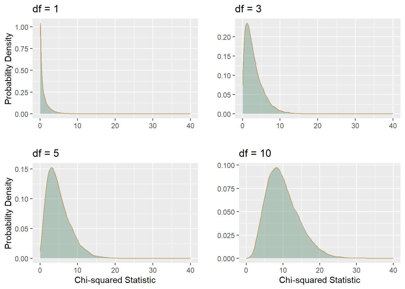
Visualizing the Chi-squared Distribution Chi-squared distribution has a single parameter, the degrees of freedom or \(df\).
\(\sqrt(2*df)\) The degrees of freedom in a chi-squared test of independence are calculated as the Number of rows−1 multiplied by Number ofcolumns−1 or more formally: \(df=(𝑟−1)∗(𝑐−1)\) The larger the contingency table, the more degrees of freedom, the wider the distribution and more normal it becomes.

The Chi-Squared Distribution is noted by:
- Right-Skewed:For low degrees of freedom, the chi-squared distribution is highly right-skewed. As the degrees of freedom increase, the skewness decreases.
- Non-Negative Values: The chi-squared distribution is defined only for non-negative values because it is the sum of squared values.
- Mean and Variance: The mean of a chi-squared distribution with k degrees of freedom is k. The variance is 2k.
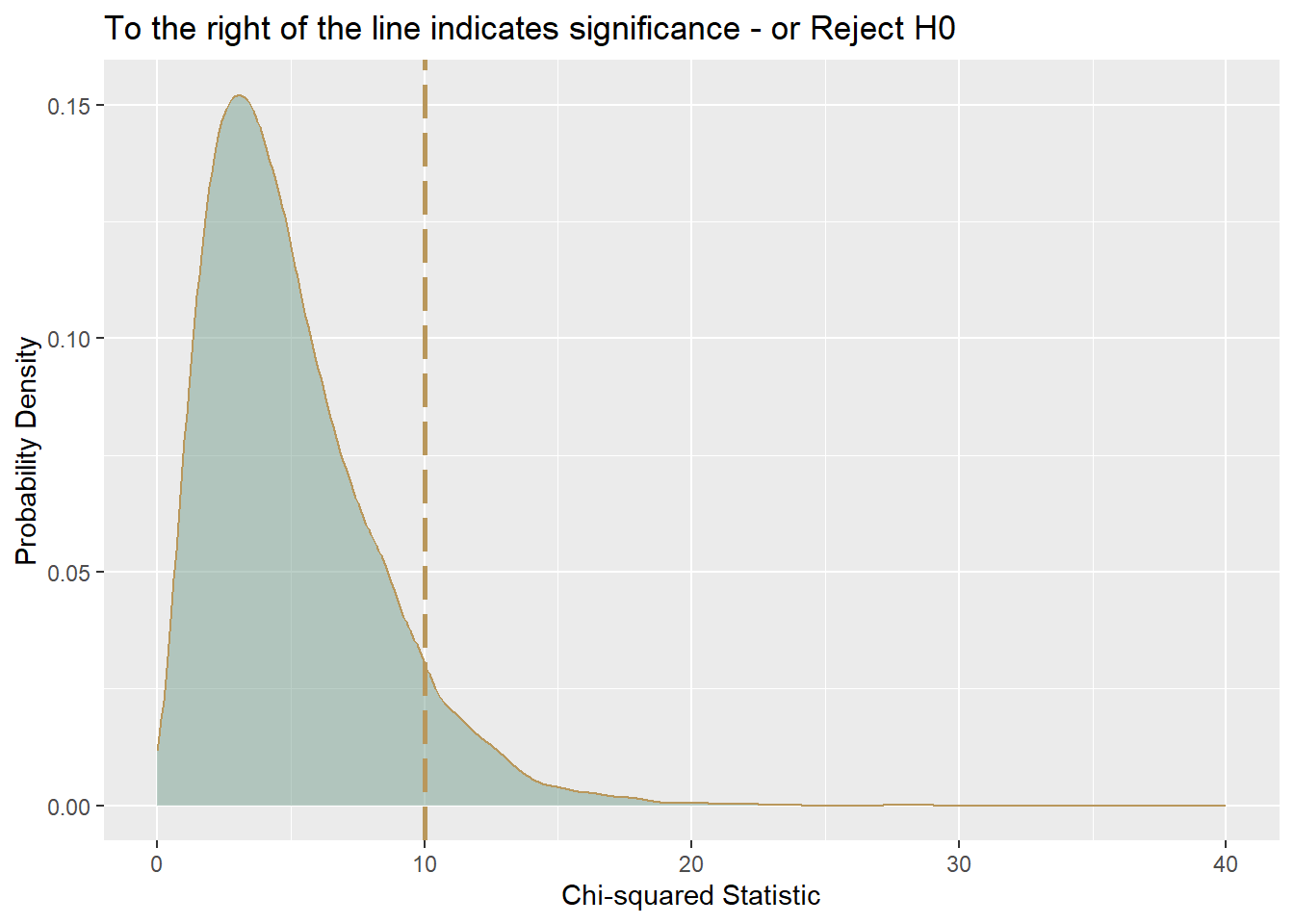
The Chi-squared probability density function shows the probability of a value of chi-squared occurring when there is no relationship between the two variables contributing to the chi-squared, where a large chi-square indicates a relationship between variables.
The competing hypotheses can be expressed as:
- \(H_0\): The two classifications are independent.
- \(H_A\): The two classifications are dependent.

Steps to conduct Chi-Squared Test for Independence

Step 1: Write the null and alternate hypotheses.
Step 2: Compute the test statistic and calculate the probability.
Step 3: State a conclusion. If the probability that the null is true is very small, usually less than 5%, reject the null hypothesis OR If the probability that the null is true is not small, usually 5% or greater, retain the null hypothesis.

Assumptions of the Chi-Squared Test of Independence

Assumption 1: The variables must be nominal or ordinal.
Assumption 2: The expected values should be 5 or higher in at least 80% of groups.
Assumption 3: The observations must be independent.
Note that there are a couple of ways observations can be non-independent.
- One way to violate this assumption would be if the data included the same set of people before and after some intervention or treatment.
- Another way to violate this assumption would be for the data to include siblings or parents and children or spouses or other people who are somehow linked to one another.
- Since people who are linked to each other often have similar characteristics, statistical tests need to be able to account for this and the chi-squared test does not.

Example of a Test for Independence

Step 1: Set up the Hypothesis
- \(H_0\): Age group and Brand Name are independent.
- \(H_A\): Age group and Brand Name are dependent.
First, we bring in the data manually from the table by column. We had 3 columns, so we need to make three vectors as shown below.

UA <- c(174, 54)
N <- c(132, 72)
A <- c(90, 78)

Then we convert these variables into a data frame. If you already have a data frame, you don’t have to do this step.

M <- data.frame(UA, N, A)
M

   UA   N  A
1 174 132 90
2  54  72 78

Always make sure your data frame looks like the table.
Step 2: Compute the test statistic and calculate the probability.
Here, we run the chisq.test() command, which only includes the columns of interest.

chisq.test(M)


    Pearson's Chi-squared test

data:  M
X-squared = 22.529, df = 2, p-value = 1.282e-05

Step 3: If the probability that the null is true is very small, usually less than 5%, reject the null hypothesis versus If the probability that the null is true is not small, usually 5% or greater, retain the null hypothesis.
Here, our p-value is 1.282e-05, so we reject the null, \(H_0\), and conclude that Age group and Brand Names are dependent.

\(df=(𝑟−1)∗(𝑐−1)\) or \((2−1)∗(3−1)=1∗2= 2df\)

Using a matrix instead of a data.frame

You can use either a matrix or a data.frame when solving a chi-squared problem.
In a Chi-squared test of independence, a matrix can be used to organize observed frequencies into categories along two dimensions. In the example, the matrix o contains data for different age groups (“Under 35” and “35 and older”) and their brand preferences (“Under Armour,” “Nike,” and “Adidas”). By setting up the matrix with these dimensions, the test evaluates whether there is a significant association between age group and brand preference. The test compares the observed counts with expected counts under the assumption that the two variables are independent.

x <- c(174, 132, 90, 54, 72, 78)
o <- matrix(x, nrow = 2, ncol = 3, byrow = TRUE)
## add some dimnames to o
dimnames(o) <- list(c("Under 35", "35 and older"), c("Under Armour", "Nike",
    "Adidas"))
o

             Under Armour Nike Adidas
Under 35              174  132     90
35 and older           54   72     78

chisq.test(o)


    Pearson's Chi-squared test

data:  o
X-squared = 22.529, df = 2, p-value = 1.282e-05

# \tPearson's Chi-squared test data: o X-squared = 22.529, df = 2,
# p-value = 0.00001282

In either case, we should see the same result. The result includes the Chi-squared statistic (X-squared = 22.529), degrees of freedom (df = 2), and a very small p-value (0.00001282), indicating a strong association between age and brand preference.

Example Using an Imported Dataset

Import the STEM data into a data frame (table) into R.
Step 1: Set up the Hypothesis:
- \(H_0\): Stem field and Gender are independent.
- \(H_A\): Stem field and Gender are dependent.

STEM <- read.csv("data/stem.csv")
STEM

   STEM.field Female Male
1    Sciences    120  100
2  Technology     15   75
3 Engineering     30  125
4        Math     15   20

Step 2: Compute the test statistic and calculate the probability.
Again, we use Rs chisq.test() command to calculate the value of the test statistic, as well as the p-value. Within the chisq.test() function, we indicate that the relevant data are in columns 2 and 3 of the data frame.

chisq.test(STEM[, 2:3])


    Pearson's Chi-squared test

data:  STEM[, 2:3]
X-squared = 66.795, df = 3, p-value = 2.072e-14

## test statistic: 66.795 df: 3 --- 4 rows and 2 columns
(4 - 1) * (2 - 1)  #3 df

[1] 3

## p-value is almost 0

Step 3: If the probability that the null is true is very small, usually less than 5%, reject the null hypothesis versus If the probability that the null is true is not small, usually 5% or greater, retain the null hypothesis.
Since the p-value is less than 0.05, we can reject the null hypothesis. At the 5% significance level, we can conclude that one’s sex does influence field choice within the STEM major.
When performing a Chi-squared test, the choice of including or excluding columns depends on which categories you want to analyze. In chisq.test(stem[, -1]), the first column is excluded, and the test is run on the remaining columns. This might be done if the first column represents data not relevant to the specific hypothesis you are testing (e.g., it could be an identifier or a control category).
On the other hand, chisq.test(stem[, 2:3]) only includes the second and third columns, focusing the analysis on specific categories of interest.
This is useful when you want to investigate the relationship between two particular variables, ignoring other columns that might be extraneous to the question you’re asking. Including or excluding columns is guided by the research hypothesis and the variables you want to test for independence.

chisq.test(STEM[, -1])  ### when we subset we use object[row, columns] --- so including the numbers 2:3 means we include variables in the 2nd and 3rd columns. Including the number -1 after the comma means that we exclude the first column.


    Pearson's Chi-squared test

data:  STEM[, -1]
X-squared = 66.795, df = 3, p-value = 2.072e-14

Chi-Squared Goodness of Fit Test

There are a few other tests regarding a Chi-squared distribution, and one other is the goodness of fit test.
This test determines whether two or more population proportions equal each other or any predetermined set of values and like the test for independence, still involves the fit between observed and estimated values.
A multinomial experiment consists of a series of n independent trials such that:
On each there are k possible outcomes.
The probability of falling into category \(i\) is the same on each trial.
The \(k\) probabilities sum to \(1:p_1 + p_2 +⋯+p_k = 1\)
The null hypothesis: the population proportions are equal to one another or they are each equal to a specific value.
For example, are four candidates in an election equally favored by voters?
Equal Population proportions:
\(H_0: P_1=P_2=P_3=P_4=.25;\)
\(H_A\):Not all populations are equal to .25
Or, do people rate food quality in a restaurant comparably to last year?
Unequal Population Proportions:
\(H_0: P_1= .4, P_2=.3, P_3= .2, P_4=.1;\)
\(H_A:\) At least one \(P_i\) differs from its hypothesized value.

Example Using Raw Numbers

Last year the management at a restaurant surveyed its patrons to rate the quality of its food. The results were as follows: 15% Excellent; 30% Good; 45% Fair; and 10% Poor.
Based on this and other survey results, management made changes to the menu.
This year, the management surveyed 250 patrons, asking the same questions about food quality. Here are the results: 46 Excellent; 83 Good; 105 Fair; and 16 Poor.
We want to know if the current results agree with those from last year, or if there has been a significant change.
To do this, we compute an expected frequency for each category and compare it to what we actually observe. Then, we compute the difference between what was observed and expected for each category. If the results this year are consistent with last year, these differences will be relatively small.
The steps are same as the Chi-Squared Test of Independence.
Step 1: Set up the Hypothesis:
- \(𝐻_0\): Each proportion equals a hypothesized value.
- \(𝐻_A\): Not all proportions equal their hypothesized values.
Step 2: Compute the test statistic and calculate the probability.
We can use R’s chisq.test() function to calculate the value of the test statistic and corresponding p-value. Within this function, we use the option p to indicate the location of the hypothesized proportions.

# Chi Squared Test Goodness of Fit
o <- c(46, 83, 105, 16)
p <- c(0.15, 0.3, 0.45, 0.1)

## quick check on p
sum(p)  ##1: sum of all proportions should be 1

[1] 1

# run the test
chisq.test(o, p = p)


    Chi-squared test for given probabilities

data:  o
X-squared = 6.52, df = 3, p-value = 0.08888

# test statistic: 6.52 df: 3 ----- 4 proportions - 1 -- or
4 - 1  ##3

[1] 3

# p-value is 0.08888 > .05

Note that p= is required here because it is not the second argument in the chisq.test() command.
Step 3: If the probability that the null is true is very small, usually less than 5%, reject the null hypothesis versus If the probability that the null is true is not small, usually 5% or greater, retain the null hypothesis.
At alpha = .05, we do not reject \(H_0\) and cannot conclude that the proportions differ from the ones a year ago.

Example Using an Imported Dataset

The steps are same as the Chi-Squared Test of Independence.
Step 1: Set up the Hypothesis:
- \(𝐻_0\): Each proportion equals a hypothesized value.
- \(𝐻_A\): Not all proportions equal their hypothesized values.
Step 2: Compute the test statistic and calculate the probability.
First, we import the stemGOF.csv data into a data frame (table) in R.
Then, again, we use Rs chisq.test function to calculate the value of the test statistic and the p-value. Within the chisq.test function, we use the option p to indicate the location of the hypothesized proportions.

STEMGOF <- read.csv("data/stemGOF.csv")
STEMGOF

            Major X2010Proportions RecentNumbers
1        Business             0.19            80
2       Education             0.09            35
3      Healthcare             0.12            85
4 Social Sciences             0.22           105
5            STEM             0.08            55
6           Other             0.30           140

chisq.test(STEMGOF$RecentNumbers, p = STEMGOF$X2010Proportions)


    Chi-squared test for given probabilities

data:  STEMGOF$RecentNumbers
X-squared = 21.526, df = 5, p-value = 0.0006441

# Chi-squared test for given probabilities data:
# stemGOF$RecentNumbers X-squared = 21.526, df = 5, p-value =
# 0.0006441 df: 6 options so 6-1 is 5 test statistic is back high:
# 21. 526

Step 3: If the probability that the null is true is very small, usually less than 5%, reject the null hypothesis versus If the probability that the null is true is not small, usually 5% or greater, retain the null hypothesis.
Since our p-value is 0.0006441, we reject \(H_0\) and conclude that the proportions differ at the 5% significance level. In this case, that means that the recent stem numbers differ from the 2010 values.

Using AI

Use the following prompts on a generative AI, like chatGPT, to learn more about probability and contingency tables.
What is a contingency table, and how is it used to represent the relationship between two categorical variables in probability calculations?
How do you calculate joint, marginal, and conditional probabilities using a contingency table, and what is the significance of each type of probability?
Can you explain how the chi-squared test for independence works, and how it is used to determine whether two categorical variables are independent or dependent?
What is the difference between the chi-squared test for independence and the chi-squared goodness of fit test, and how is each test applied?
Once you calculate the chi-squared test statistic, how do you interpret the p-value to determine whether to reject or fail to reject the null hypothesis?
Why are degrees of freedom important in a chi-squared test, and how do you calculate them for a contingency table?
How do you set up and execute a chi-squared test using the chisq.test() function in R, and what are the key outputs to focus on when interpreting the results?

Summary

In this lesson, we learned about contingency tables in regards to calculating probability with two categorical variables. We also computed the chi-squared statistics for the test of independence and the goodness of fit.
We note that the “Goodness of fit” and “test of independence” are both chi-square tests, but they serve different purposes:
Goodness of Fit test: Purpose: Assesses how well observed data match a specified distribution (often a theoretical or expected distribution). Example: Checking if the distribution of colors of M&M’s in a bag matches the expected company distribution (say, 30% blue, 20% red, etc.). Null Hypothesis: The observed frequencies match the expected frequencies.
Test of Independence: Purpose: Determines whether there is a significant association between two categorical variables in a contingency table. Example: Evaluating if gender (male/female) is independent of preference for a type of product (e.g., A or B). Null Hypothesis: The two variables are independent (no association).