####################################
# Project name: Module 1
# Project purpose: To create an R script file to learn about R.
# Code author name: [Enter Your Name]
# Date last edited: [Enter Date Here]
# Data used: NA
# Libraries used: NA
####################################Introduction to Analytics using R and AI
This lesson introduces R and RStudio — the statistical computing environment used throughout this course — alongside the generative AI concepts you will rely on from your first assignment onward. By the end, you will be able to navigate RStudio, write and run R code, create and name objects, load data from external files, and use AI tools responsibly.
We begin with the foundations of statistics and AI: what descriptive and inferential statistics are, where AI fits into each branch, and what it means to be fluent in R in an age when AI can write code on demand. Understanding the “why” behind each command is what separates an analyst from someone who just runs code.
We then move to understanding generative AI: how large language models work mechanically, what they handle reliably versus what they get wrong, how hallucinations arise and what warning signs to watch for, and how to write effective prompts for R and statistics tasks. These concepts apply to every AI interaction throughout the course and are built on directly in the Generative AI and Data Visualization lesson.
We then move to setting up and using R: creating script files, writing comments and a prolog, performing arithmetic, assigning values to objects, naming those objects consistently, working with built-in functions, installing and loading packages, and troubleshooting errors. These are the mechanical building blocks every subsequent lesson relies on.
We close with entering and loading data: building vectors, matrices, and data frames from scratch, setting a working directory, and reading in external files with read.csv() and read_csv(). Understanding the difference between absolute and relative file paths — and why relative paths are preferred — is a practical skill that prevents a large share of beginner errors.
By the end of this lesson, you should be comfortable writing and running basic R code, loading a dataset, and applying the hallucination warning signs and prompting strategies to AI-generated output. Data types, coercion, and missing data handling are covered in depth in the Data Preparation lesson, where they are taught alongside real cleaning workflows. Work through every code example in your own .R script file alongside the reading.
At a Glance
- In order to succeed in this lesson, you will need to have both R and RStudio downloaded and open. The only way to learn R is to use it — type every code example yourself rather than just reading it. Pay attention not just to what you are typing but why the code is written that way, and what other forms would produce the same result.
- This is a statistics course, and R is a statistical computing tool. The two are inseparable here. Every command you learn connects to a statistical concept, and understanding that connection is what makes the code meaningful rather than mechanical.
- The generative AI section is not a detour — it is prerequisite knowledge for using AI tools responsibly throughout the course. Pay close attention to the hallucination warning signs and the three-step verification check; you will apply both in every subsequent lesson.
Lesson Objectives
- Explain the difference between descriptive and inferential statistics and identify where AI assists versus where human judgment is required.
- Describe how large language models work at a mechanical level (tokenization, attention mechanisms, language prediction vs. truth verification).
- Identify the five hallucination warning signs and apply the three-step verification check to AI-generated R output.
- Write effective zero-shot, few-shot, and chain-of-thought prompts for R and statistics tasks.
- Create and run an R script file with a prolog, comments, and code.
- Assign values to objects using the
<-operator and follow consistent naming conventions. - Use built-in functions with single and multiple arguments, including default values.
- Install and load packages; access functions using the
library::function()syntax. - Troubleshoot common R errors using a systematic approach.
- Create vectors, matrices, and data frames from scratch.
- Set a working directory and load data using
read.csv()andread_csv(). - Load a dataset, run
str()andsummary()to inspect it, and access columns with$.
Consider While Reading
- In the generative AI section, focus on the mechanical explanation of how LLMs work — not to become an AI engineer, but because understanding that the model is predicting language (not computing truth) changes how you read and verify its output. The hallucination warning signs follow directly from this mechanism.
- R has a steep learning curve, but the curve flattens fast once you start recognising patterns. Every error message is information — read it before asking AI to fix it. Every function has a help page — check it before guessing at arguments.
- As you read, notice how the lesson is structured as a workflow: statistics foundations → generative AI → set up R → write code → create data → load data. Each section is a prerequisite for the next.
- AI tools like ChatGPT and GitHub Copilot can write R code for you. The goal of this lesson is to build enough understanding that you can read, verify, and own that code — not just run it and hope for the best.
What is Statistics?
- Statistics is the methodology of extracting useful information from a data set.
- Numerical results are not very useful unless they are accompanied with clearly stated actionable business insights.
- To do good statistical analysis, you must do the following:
- Find the right data.
- Use the appropriate statistical tools.
- Clearly communicate the numerical information in written language.
- With knowledge of statistics:
- Avoid risk of making uninformed decisions and costly mistakes.
- Differentiate between sound statistical conclusions and questionable conclusions.
- Data and analytics capabilities have made a leap forward.
- Growing availability of vast amounts of data.
- Improved computational power.
- Development of sophisticated algorithms.
- The rise of Generative AI.
Definition of AI
- Artificial Intelligence (AI) is the development of computer systems that can perform tasks that typically require human intelligence — things like recognizing patterns, making decisions, understanding language, and generating content.
- For the purposes of this course, the most relevant category is generative AI (tools like ChatGPT, Claude, and GitHub Copilot), which can produce text, code, and analysis in response to natural language prompts.
The AI Landscape: Where Generative AI Fits
AI is not a single thing — it is a nested set of capabilities, and understanding where generative AI sits within that hierarchy helps you use it more effectively and avoid overstating what it can do.
Artificial Intelligence is the broad effort to create systems that can mimic human intelligence — reasoning, learning, adapting. Within that, Machine Learning is one of the most important approaches: algorithms that learn from data to make predictions or recommendations. When Netflix suggests your next show or a bank predicts loan default risk, that is machine learning at work.
A subset of ML is Deep Learning — neural networks with many layers that power image recognition, speech recognition, and voice assistants. And within deep learning sits Generative AI, which represents a new kind of capability: instead of classifying or predicting, generative models create — producing text, images, code, and audio that did not exist before.
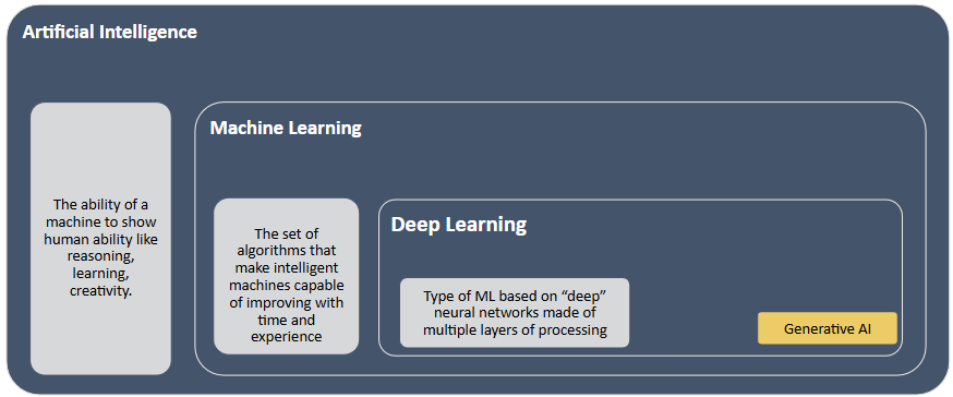
Generative AI refers specifically to AI systems that create new content — text, code, images, audio, and video — based on patterns learned from training data. It is distinct from predictive AI, which forecasts outcomes from historical data without producing new content.
| Type | Goal | Business example |
|---|---|---|
| Generative AI | Create new content | Drafting a report, writing R code, generating chart titles |
| Predictive AI | Forecast outcomes | Customer churn model, demand forecasting, credit scoring |
Both types are useful in a statistics course. Predictive AI is what you are building when you run a regression. Generative AI is what helps you write, code, and communicate. Understanding the difference prevents misuse.
Notable tools in a business statistics context: ChatGPT and Claude (text and code generation), GitHub Copilot (code completion in your editor), and Perplexity AI (search combined with generative synthesis).
Narrow AI, General AI, and Strong AI
Generative AI feels general because it handles so many different kinds of tasks. But even the most capable tools like ChatGPT or Claude are still forms of Narrow AI — systems designed to perform well within a defined domain without genuine general reasoning.
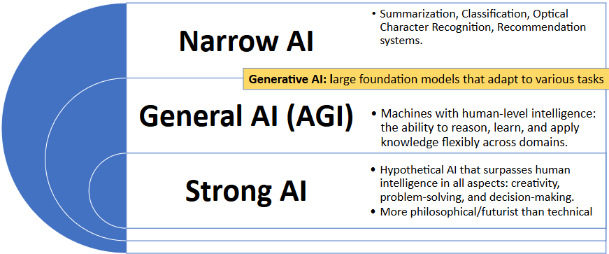
The three levels of AI capability are:
- Narrow AI — systems designed to do one thing, or a small set of related tasks, extremely well. Spam filters, recommendation engines, facial recognition, and medical imaging classifiers are all narrow AI. Generative AI tools belong here too — they are extraordinarily capable within the domain of language, but they do not generalize outside it the way a human reasoner does.
- General AI (AGI) — a hypothetical system that could understand, learn, and apply knowledge across any domain at human level or beyond. AGI remains aspirational.
- Strong AI — a further hypothetical: AI that surpasses human intelligence across all domains, including creativity, problem-solving, and decision-making.
You can think of generative AI as broad narrow AI: remarkably versatile within the domain of language and content generation, but still limited outside of it. A large language model cannot reason about an entirely new domain the way a human expert can — it pattern-matches against its training data.
Two Main Branches of Statistics
- Descriptive Statistics - collecting, organizing, and presenting the data.
- Inferential Statistics - drawing conclusions about a population based on sample data from that population.
- A population consists of all items of interest.
- A sample is a subset of the population.
- A sample statistic is calculated from the sample data and is used to make inferences about the population parameter.
- Reasons for sampling from the population:
- Too expensive to gather information on the entire population.
- Often impossible to gather information on the entire population.
Descriptive Statistics and AI
- Descriptive Statistics is where AI currently dominates. Tools like ChatGPT, Copilot, and R’s own AI-assisted packages can collect data via APIs, clean and wrangle it, generate summary statistics, and produce polished visualizations faster than any human. When you ask AI to “summarize this dataset,” it’s doing descriptive work. The output is only as good as the data fed in, but the mechanical execution is largely automated.
Inferential Statistics and AI
- Inferential Statistics is where human judgment remains essential, and AI actually introduces new complications. Consider:
- Who defines the population? If you’re studying customer behavior, do you mean all customers, all potential customers, all customers in a region? AI won’t ask this question — it will answer whatever you give it. Defining the population of interest is a business and conceptual judgment call, not a computation.
- Is the sample representative? AI can run a regression or t-test in seconds, but it cannot tell you whether your sample was collected with selection bias, convenience sampling, or missing key subgroups. That requires domain knowledge and critical thinking.
- What do the inferences actually mean? A p-value of 0.03 in a business context means something different from one in a clinical trial. Translating statistical conclusions into actionable decisions — and communicating uncertainty honestly to a non-technical audience — is still entirely a human skill.
AI and the Analytics Workflow
Before diving into R, it is worth situating AI within the broader analytics workflow you will encounter throughout this course and in business settings. Traditional analytics follows a familiar progression:
- Descriptive analytics — what happened (reports, summaries, visualizations)
- Diagnostic analytics — why it happened (exploring relationships and causes)
- Predictive analytics — what will happen (forecasting models, regression)
- Prescriptive analytics — what we should do (recommendations, optimization)
These four categories have shaped how organizations approach data for decades, and they remain the core of what you are learning in this course. AI does not replace this progression — it supercharges it. AI makes the traditional analytics cycle faster, deeper, and more dynamic. The key distinction for this course is between AI as a tool you use and AI as a system an organization embeds. When you use Claude or ChatGPT to write R code or interpret output, you are using AI as a productivity tool — it handles mechanical execution while you supply the question, the data, and the judgment. You will return to this framework throughout the course as you move from descriptive statistics all the way through regression.
Understanding Generative AI
How Generative AI Works: A Conceptual Overview
Generative AI systems — specifically large language models (LLMs) like GPT-4 and Claude — are trained on massive text corpora to predict the most likely next word given a sequence of prior words. This sounds simple, but at sufficient scale (billions of parameters, trillions of training tokens) it produces systems capable of reasoning, code generation, summarization, and dialogue.
Two concepts explain most of what you will observe when using these tools:
Tokenization — the model does not read words; it reads tokens, which are chunks of text (often subwords). “Unbelievable” might become ["un", "believ", "able"]. The model learns statistical relationships between token sequences across enormous amounts of text.
Attention mechanisms — instead of processing text strictly left-to-right, the model can attend to any prior token when predicting the next one. This is what allows it to understand that “bank” means something different in “river bank” and “savings bank.”
The key insight for a business analyst: the model is predicting language, not computing truth. When it writes mean(x) = sum(x) / length(x), it is not running a calculation — it is recognizing that this string follows that kind of prompt in training data. Usually this is correct. Sometimes it is not.
The Limits of Generative AI
Understanding what AI does reliably versus what it struggles with is the most practical thing in this section.
| AI handles well | Requires your judgment |
|---|---|
| Writing and editing code syntax | Verifying that the code answers your question |
| Generating chart boilerplate | Evaluating whether the chart is analytically honest |
| Summarizing text and documents | Checking whether the summary is accurate |
| Explaining statistical concepts | Deciding whether the explanation applies to your context |
| Formatting and structuring output | Determining whether the structure serves your audience |
| Arithmetic in simple expressions | Any multi-step calculation (AI approximates, not computes) |
AI Hallucinations: What to Watch For Before You Start
Because you will be using AI to help write and debug R code from your very first assignment, it is important to understand one critical limitation before you begin: hallucinations.
Hallucinations occur when an LLM generates plausible-sounding but factually incorrect content. The model does not know it is wrong — it produces the statistically most likely continuation of the prompt, which can be entirely fabricated. A well-known example: a lawyer asked ChatGPT to provide legal cases supporting an argument. The model returned several cases with plausible names, courts, years, and rulings. None of them existed.
Hallucinations are not a fixable bug — they are a structural property of how language prediction works. When the correct answer is rare or absent in training data, the model produces whatever is statistically likely, not whatever is true.
Five warning signs to watch for in every AI response:
| Warning sign | Example |
|---|---|
| Unverified specificity | Exact statistics cited without a source |
| Invented sources | Journal articles, packages, or functions that do not exist |
| Internal contradictions | Two claims within the same response that conflict |
| Overconfident language | “This is definitively true” on an uncertain topic |
| Failures of common sense | Physically or logically impossible claims |
Practical rule: always run and verify AI-generated R code yourself. Never submit code you have not executed and checked.
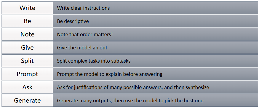
Prompt Engineering: Getting Better Output from AI
Because you will be using AI to write and debug R code throughout this course, the quality of what AI returns depends directly on the quality of what you ask.
Prompt engineering is the practice of crafting inputs to elicit reliable, specific outputs from AI systems. The core principle is direct: the quality of the prompt determines the quality of the response. A vague prompt produces a vague answer.
Three prompting strategies — each suited to different types of tasks:
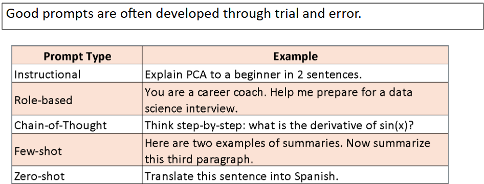
Zero-shot prompting — give the task with no examples. Works well for straightforward requests where the task is clear.
“Classify this customer review as positive, negative, or neutral: ‘The delivery was two days late and the packaging was damaged.’”
Few-shot prompting — provide a small number of labeled examples before the target request. Useful when the format or classification scheme needs to be demonstrated.
“Classify each as positive, negative, or neutral. ‘Great service, arrived early’ → positive ‘Wrong item sent’ → negative *‘Package arrived on time’ → ___“*
Chain-of-thought prompting — instruct the model to reason through steps before answering. Significantly improves accuracy on multi-step or ambiguous tasks.
“Classify the following review as positive, negative, or neutral. Think step by step: first identify the key sentiment signals, then determine the overall tone, then give your classification. Review: ‘The product quality is fine but customer support never responded to my three emails.’”
For R and statistics tasks, specificity is the most important lever. Compare these prompts:
| Vague prompt | Specific prompt |
|---|---|
| “Make a chart of my data” | “Using ggplot2, create a bar chart of mean home_value by season from zillow.csv. Use fill to color by season, sort bars from highest to lowest mean, and label the y-axis in dollars.” |
| “Run a t-test” | “Run a two-sample t-test comparing home_value between Summer and Winter observations in zillow.csv. State the hypotheses, run t.test(), and interpret the p-value at α = 0.05.” |
| “What does this output mean?” | “I ran summary(lm(home_value ~ season, data=zillow)) and got these results: [paste output]. Explain what the Intercept, seasonSpring coefficient, and p-values mean in plain English for a non-statistician.” |
Verifying AI output — a three-step check you will use all semester:
- Run the code — does it execute without errors?
- Sanity-check the output — do the numbers make sense given what you know about the data?
- Verify the interpretation — does the AI’s explanation match the statistical meaning of the output?
Step 3 is where statistical knowledge is irreplaceable. AI can produce a confidence interval and write a plausible-sounding sentence about it — but you need to know whether the sentence is correct. You will apply these strategies throughout the course; the Generative AI and Data Visualization chapter will build on them further.
What makes you fluent in R — with or without AI:
The skills that matter most in this course — and that AI cannot fully substitute for — are: troubleshooting errors by reading them carefully, understanding the environment and what objects are loaded, using the assignment operator and built-in functions correctly, reading data, loading packages, and prompting and verifying AI-generated code. R is also a dynamically typed language, meaning it figures out a variable’s data type automatically based on what you assign to it — you do not have to declare types upfront, but you do have to check them, which is covered in the Data Types section below.
Setting up R
R Script Files
- Using R Script Files:
- A .R script is simply a text file containing a set of commands and comments. The script can be saved and used later to rerun the code. The script can also be documented with comments and edited again and again to suit your needs.
- Using the Console
- Entering and running code at the R command line is effective and simple. However, each time you want to execute a set of commands, you must re-enter them at the command line. Nothing saves for later.
- Complex commands are particularly difficult, forcing you to re-enter the code to fix any errors — typographical or otherwise. R script files help to solve this issue.
Create a New R Script File
- To save your notes from this lesson, create a .R file named module1.R and save it to your project file you made in the last class.
- There are a couple of parts to this module, and we can add code for the entire module in one file so that our code is stacked nicely together.
- For each new module, start a new file and save it to your project folder.

With R installed and a script file open, it is time to start writing code. This section introduces the core mechanics of the R language: comments, arithmetic, objects, naming conventions, built-in functions, packages, and how to troubleshoot when something goes wrong.
Using R
Text in R
A Prolog
- A prolog is a set of comments at the top of a code file that provides information about what is in the file. It also names the files and resources used that facilitates identification. Including a prolog is considered coding best practice.
- On your own R Script File, add your own prolog following the template as shown.
- An informal prolog is below:
- Then, as we work through our .R script and add data files or libraries to our code, we go back and edit the prolog.

String
- In R, a string is a sequence of characters enclosed in quotes, used to represent text data.
- R accepts single quotes or double quotes when marking a string. However, if you use a single quote to start, use a single quote to end. The same for double quotes - ensure the pairing is the same quote type.
- You sometimes need to be careful with nested quotes, but generally it does not matter which you use.
"This is a string"[1] "This is a string""This is also a string"[1] "This is also a string"Note on R Markdown: These lesson files are formatted with RMarkdown. When you see R code followed by output in this document, you only need to type the code itself into your
.Rscript file. The RMarkdown lesson covers this format in full detail.
Running Commands
- There are a few ways to run commands via your .R file.
- You can click Ctr + Enter on each line (Cmd + Return on a Mac).
- You can select all the lines you want to run and select Ctr + Enter (Cmd + Return on a Mac).
- You can select all the lines you want to run and select the run button as shown in the Figure.

- Now that I have asked you to add a couple lines of code, after this point, when R code is shown on this file, you should add it to your .R script file along with any notes you want. I won’t explicitly say - “add this code.”
R is an Interactive Calculator
- An important facet of R is that it should serve as your sole calculator.
- Try these commands in your .R file by typing them in and clicking Ctr + Enter on each line for a PC and Cmd + Return on a Mac computer.
3 + 4[1] 73 * 4[1] 123/4[1] 0.753 + 4 * 100^2[1] 40003- Take note that order of operations (PEMDAS) holds in R: parentheses first, then exponents, then multiplication/division and modulo (
%%) left to right, then addition/subtraction. When in doubt, use parentheses to make the intended order explicit.
# R respects standard order of operations
3 + 4 * 100^2  # exponent first, then multiply, then add
[1] 400032 + 3 * 5 - 7^2%%4 + (5/2) # = 18.5[1] 18.5Creating Objects
- Entering and Storing Variables in R requires you to make an assignment.
- We use the assignment operator ‘<-’ to assign a value or expression to a variable.
- We typically do not use the = sign in R even though it works because it also means other things in R.
- Some examples are below to add to your .R file.
states <- 29
A <- "Apple"
# Equivalent statement to above - again = is less used in R.
A = "Apple"
print(A)
[1] "Apple"# Equivalent statement to above
A[1] "Apple"B <- 3 + 4 * 12
B[1] 51
Naming Objects
- Line length limit: 80
- Always use a consistent way of annotating code.
- Camel case is capitalizing the first letter of each word in the object name, with the exception of the first word.
- Dot case puts a dot between words in a variable name while camel case capitalizes each word in the variable name.
- Object names appear on the left of assignment operator. We say an object receives or is assigned the value of the expression on the right.
- Naming Constants: A Constant contains a single numeric value.
- The recommended format for constants is starting with a “k” and then using camel case. (e.g., kStates).
- Naming Functions: Functions are objects that perform a series of R commands to do something in particular.
- The recommended format for Functions is to use Camel case with the first letter capitalized. (e.g., MultiplyByTwo).
- Naming Variables: A Variable is a measured characteristic of some entity.
The recommended format for variables is to use either the dot case or camel case. e.g., filled.script.month or filledScriptMonth.
A valid variable name consists of letters, numbers, along with the dot or underline characters.
A variable name must start with a letter, or the dot when not followed by a number.
A variable cannot contain spaces.
Variable names are case sensitive: x is different from X just as Age is different from AGE.
The value on the right must be a number, string, an expression, or another variable.
Some Examples Using Variable Rules:
AB.1 <- "Allowed?"
# Does not follow rules - not allowed Try the statement below with no
# hashtag to see the error message .123 <- 'Allowed?'
A.A123 <- "Allowed?"
G123AB <- "Allowed?"
# Recommended format for constants
kStates <- 29
The naming conventions above can be summarised as:
| Object type | Convention | Example |
|---|---|---|
| Constant (single value) | k + CamelCase |
kStates, kMaxRetries |
| Function | CamelCase, first letter capitalised | MultiplyByTwo, CleanData |
| Variable / column | dot.case or camelCase | filled.script.month, filledScriptMonth |
| Dataset / data frame | Short, lowercase or camelCase | gig, gss.2016, potLegal |
- Different R coders have different preferences, but consistency is key in making sure your code is easy to follow and for others to read. In this course, we will generally use the recommendation in the text which are listed above.
- We tend to use one letter variable names (i.e., x) for placeholders or for simple functions (like naming a vector).
Built-in Functions
- R has thousands of built-in functions including those for summary statistics. Below, we use a few built-in functions with constant numbers. The sqrt(), max(), and min() functions compute the square root of a number, and find the maximum and minimum numbers in a vector.
sqrt(100)[1] 10max(100, 200, 300)[1] 300min(100, 200, 300)[1] 100We can also create variables to use within built-in functions.
Below, we create a vector x and use a few built-in functions as examples.
- The sort() function sorts a vector from small to large.
x <- c(1, 2, 3, 3, 100, -10, 40)  #Creating a Vector x
sort(x)  #Sorting the Vector x from Small to Large
[1] -10 1 2 3 3 40 100max(x) #Finding Largest Element of Vector x[1] 100min(x) #Finding Smallest Element of Vector x[1] -10
Built-in Functions: Setting an Argument
- The standard format to a built-in function is functionName(argument)
- For example, the square root function structure is listed as sqrt(x), where x is a numeric or complex vector or array.
# Here, we are setting a required argument x to a value of 100. When
# a value is set, it turns it to a parameter of the function.
sqrt(x = 100)
[1] 10# Because there is only one argument and it is required, we can
# eliminate its name x= from our function call. This is discussed
# below.
sqrt(100)[1] 10- There is a little variety in how we can write functions to get the same results.
- A parameter is what a function can take as input. It is a placeholder and hence does not have a concrete value. An argument is a value passed during function invocation.
- There are some default values set up in R in which arguments have already been set.
- There are a few functions with no parameters like Sys.time() which produces the date and time. If you are not sure how many parameters a function has, you should look it up in the help.
Default Values
- There are many default values set up in R in which arguments have already been set to a particular value or field.
- Default values have been set when you see the = value in the instructions. If we don’t want to change it, we don’t need to include it in our function call.
- When only one argument is required, the argument is usually not set to have a default value.
Built-in Functions: Using More than One Argument
- For functions with more than one parameter, we must determine what arguments we want to include, and whether a default value was set and if we want to change it. Default values have been set when you see the = value in the instructions. If we don’t want to change it, we don’t need to include it in our function call.
- For example, the default S3 method for the seq() function is listed as the following: seq(from = 1, to = 1, by = ((to - from)/(length.out - 1)),length.out = NULL, along.with = NULL, …)
- Default values have been set on each parameter, but we can change some of them to get a meaningful result.
- For example, we set the from, to, and by parameter to get a sequence from 0 to 30 in increments of 5.
# We can use the following code.
seq(from = 0, to = 30, by = 5)
[1] 0 5 10 15 20 25 30We can simplify this function call even further:
- If we use the same order of parameters as the instructions, we can eliminate the argument= from the function.
- Since we do list the values to the arguments in same order as the function is defined, we can eliminate the from=, to=, and by= to simplify the statement.
# Equivalent statement as above
seq(0, 30, 5)
[1] 0 5 10 15 20 25 30If you leave off the by parameter, it defaults at 1.
# Leaving by= to default value of 1
seq(0, 30)
[1] 0 1 2 3 4 5 6 7 8 9 10 11 12 13 14 15 16 17 18 19 20 21 22 23 24
[26] 25 26 27 28 29 30- There can be a little hurdle deciding when you need the argument value in the function call. The general rule is that if you don’t know, include it. If it makes more sense to you to include it, include it.
Tips on Arguments
- Always look up a built-in function to see the arguments you can use.
- Arguments are always named when you define a function.
- When you call a function, you do not have to specify the name of the argument.
- Arguments have default values, which is used if you do not specify a value for that argument yourself.
- An argument list comprises of comma-separated values that contain the various formal arguments.
- Default arguments are specified as follows: parameter = expression
y <- 10:20
sort(y)
[1] 10 11 12 13 14 15 16 17 18 19 20sort(y, decreasing = FALSE) [1] 10 11 12 13 14 15 16 17 18 19 20The Environment
- You can evaluate your Environment Tab to see your Variables we have defined in R Studio.
- Use the following functions to view and remove defined variables in your Global Environment
ls() #Lists all variables in Global Environment [1] "A" "A.A123" "AB.1" "B" "G123AB" "kStates" "states"
[8] "x" "y" rm(states) #Removes variable named states
rm(list = ls()) #Clears all variables from Global Environment
Saving
- You can save your work in the file menu or the save shortcut using Ctrl + S or Cmd + S depending on your Operating System.

Installing a Package and Calling a Library
- A package is a collection of functions, data, and code. The library is where packages live
- We use the install.package command one time to install a package.
- tidyverse is a collection of packages designed to work together for data import, cleaning, and visualization. Loading one line gives you all of them.
- You can also install via the menu: Tools > Install Packages — type the package name and click Install. Same result, no typing required.
- Then, we use the library command to load the library.
- When tidyverse loads, R will tell you exactly which packages were attached and which functions now have conflicts. Read that message — it tells you something important about your environment.
# Install once — ever. After that, comment this line out.
# install.packages('tidyverse') ##commented out for processing

# Load every R session
library(tidyverse)
A Common Mistake
Leaving install.packages() uncommented in your script means R reinstalls the package every time you run the file. That wastes time and can cause version issues. Comment it out after the first run.
# install.packages('tidyverse') # commented out after install
library(tidyverse) # this is all you need going forward- If a package won’t load, the fix is almost always one of these:
- You never installed it — run install.packages() once
- You forgot library() at the top of your script
- There is a typo — package names are case sensitive
Accessing A Function from Specific Library
- You can access a function from a specific library using the double-colon operator library::function()
- Useful if only using one function from the library.
- We will return to this in data prep.
## Below is an example that would use dplyr for one select function
## to select variable1 from the oldData and save it as a new object
## NewData. Since we don’t have datasets yet, we will revisit this.
## NewData <- dplyr::select(oldData, variable1)- Some libraries are part of other global libraries:
- dplyr is part of tidyverse, there is actually no need to activate it if tidyverse is active, however, sometimes it helps when conflicts are present
- An example of a conflict is the use of a select function which shows up in both the dplyr and MASS package. If both libraries are active, R does not know which to use.
- tidyverse has many libraries included in it.
Troubleshotting Errors in RStudio
- Step 1: Restart RStudio/Restart Computer and Clear your environment
- Use rm(list=ls()) to clear out old variables
- Make sure proper capitalization and spacing is being used.
- Step 2: Read the error message carefully: R’s error messages are more informative than they look. Check capitalization, spelling, and whether all parentheses and quotes are closed. Most beginner errors live here.
- Step 3: Ask AI: Paste the error message directly into ChatGPT or Claude and ask what it means. This is a legitimate and efficient use of AI — error interpretation is exactly what it is good at.
- Verify the fix yourself before running it. AI can suggest plausible-looking code that does the wrong thing.
- Three-step check for any AI-generated R code: (1) Run the code — does it execute without errors? (2) Sanity-check the output — do the numbers make sense given what you know about the data? (3) Verify the interpretation — does the AI’s explanation actually match the statistical meaning of the output? Step 3 is where your growing statistical knowledge is irreplaceable — AI can produce a result and write a plausible sentence about it, but only you can confirm that sentence is correct.
- Two Categories of Errors (Both Matter Equally)
- Hard Error: Code won’t run at all (Easy to catch)
- Silent Error: Code runs but gives wrong output (Dangerous – easy to miss)
- The second type is the more important one to develop instincts for. AI is particularly prone to silent errors — it will produce output that looks correct but isn’t. Always sanity-check results against what you expect.
With the language mechanics established, the next step is creating data structures directly in R. Before you read in real datasets, understanding how vectors, matrices, and data frames are built from scratch gives you a mental model of how R stores and organises data.
Entering Data in R
Creating a Vector
- A vector is the simplest type of data structure in R.
- A vector is a set of data elements that are saved together as the same type.
- We have many ways to create vectors with some examples below.
- Use c() function, which is a generic function which combines its arguments into a vector or list.
c(1, 2, 3, 4, 5) #Print a Vector 1:5[1] 1 2 3 4 5- If numbers are aligned, can use the “:“ symbol to include numbers and all in between. This is considered an array.
1:5 #Print a Vector 1:5[1] 1 2 3 4 5- Use seq() function to make a vector given a sequence.
seq(from = 0, to = 30, by = 5) #Creates a sequence vector from 0 to 30 in increments on 5 [1] 0 5 10 15 20 25 30- Use rep() function to repeat the elements of a vector.
rep(x = 1:3, times = 4) #Repeat the elements of the vector 4 times [1] 1 2 3 1 2 3 1 2 3 1 2 3rep(x = 1:3, each = 3) #Repeat the elements of a vector 3 times each[1] 1 1 1 2 2 2 3 3 3The four main ways to create a vector in R:
| Function | Purpose | Example | Result |
|---|---|---|---|
c() |
Combine any values | c(1, 2, 3) |
1 2 3 |
: |
Integer sequence | 1:5 |
1 2 3 4 5 |
seq() |
Custom sequence with step | seq(0, 30, 5) |
0 5 10 … 30 |
rep() |
Repeat elements | rep(1:3, times=2) |
1 2 3 1 2 3 |
Creating a Matrix
A matrix is a rectangular object with rows and columns where every element must be the same data type (usually numeric). In practice, you will almost always work with data frames rather than matrices in this course — but understanding the distinction matters: a data frame allows mixed column types (a character column next to a numeric column); a matrix does not.
# Create a 3x3 matrix filled column-by-column by default
x <- 1:9
matrix(x, nrow = 3, ncol = 3)
[,1] [,2] [,3]
[1,] 1 4 7
[2,] 2 5 8
[3,] 3 6 9Creating a Data Frame
A data frame is a table or a two-dimensional array-like structure in which each column contains values of one variable and each row contains one set of values from each column. In a data frame the rows are observations and columns are variables.
- Data frames are generic data objects to store tabular data.
- The column names should be non-empty.
- The row names should be unique.
- The data stored in a data frame can be of numeric, factor or character type.
- Each column should contain same number of data items.
- Combing vectors into a data frame using the data.frame() function
Going back to the basics in statistics, we need to define an observation and variable so that we can know how to use them effectively in R in creating data frame objects.
An Observation is a single row of data in a data frame that usually represents one person or other entity.
A Variable is a measured characteristic of some entity (e.g., income, years of education, sex, height, blood pressure, smoking status, etc.).
In data frames in R, the columns are variables that contain information about the observations (rows).
Below, we can create vectors for state, year enacted, personal oz limit medical marijuana.
state <- c("Alaska", "Arizona", "Arkansas")
year.legal <- c(1998, 2010, 2016)
ounce.lim <- c(1, 2.5, 3)- Then, we can combine the 3 vectors into a data frame and name the data frame pot.legal.
pot.legal <- data.frame(state, year.legal, ounce.lim)- Next, check your global environment to confirm data frame was created.

Observations: States being measured.
Variables: Information about each state (State Name, Year Weed was legalized, and the Ounce Limit permitted).
# Shows the number of columns or variables
ncol(pot.legal)
[1] 3# Shows the number of rows or observations
nrow(pot.legal)[1] 3# Shows both the number of rows (observations and columns
# (variables).
dim(pot.legal)[1] 3 3You can build data manually, but most real analysis starts with loading an external file. Before reading data into R, you need to understand where R looks for files — which is what working directories and file paths control.
Working Directories
In R, when working with data files stored on your computer, it’s important to understand the difference between absolute and relative file paths. An absolute reference gives the complete path to the file, starting from the root directory. This path is specific to your system, and it doesn’t change regardless of where the R script is located. For example, on a Windows machine, you might use something like
read.csv("C:/Users/username/Documents/data.csv"). This path will always point to the same file, but it can make your code less portable since it only works on your machine or if others have the exact same file structure.On the other hand, a relative reference specifies the file’s path relative to the location of your R script or working directory. It is more flexible because it assumes the file is located in a directory relative to the current project or script. For example, if your script and data file are in the same folder, you could use
read.csv("data.csv"). If the file is in a subdirectory, you would reference it relatively likeread.csv("data/data.csv"). Relative paths make your code more portable and easier to share since it will work as long as the folder structure remains consistent.Using relative paths is often a best practice, especially in collaborative projects or when sharing code. You can check your current working directory in R with
getwd()and set it withsetwd().
Absolute File Paths
- Absolute vs. Relative Links
- An absolute file path provides the complete location of a file, starting from the root directory of your computer.
- Always points to the same file.
- Independent of the script’s location.
- Example:
read.csv("C:/Users/username/Documents/data.csv")
- Pro
- Reliable for your system
- No Ambiguity in locating files
- Cons
- Not portable; requires the same file structure across systems.
- Harder to share code with collaborators.
Relative File Paths
- A relative file path specifies the file location based on the working directory of your R project or script.
- Changes based on the working directory.
- Often starts from the project folder.
- Example:
read.csv("data/myfile.csv")
- Pros
- More portable; works across systems if the project structure is consistent.
- Easier collaboration when sharing code and project files.
- Cons
- Requires setting the working directory correctly (getwd() and setwd() can help).
| Absolute path | Relative path | |
|---|---|---|
| Example | "C:/Users/pam/Documents/data.csv" |
"data/data.csv" |
| Starts from | Root of the file system | Current working directory |
| Portability | Breaks on any other machine | Works on any machine with the same folder structure |
| Best for | Quick personal scripts | Shared projects, submitted work |
Setting up a Working Directory
You should have the data files from our LMS in a data folder on your computer. Your project folder would contain that data folder.
Before importing and manipulating data, you must find and edit your working directory to directly connect to your project folder!
These functions are good to put at the top of your R files if you have many projects going at the same time.
getwd()  #Alerts you to what folder you are currently set to as your working directory
# For example, my working directory is set to the following:
# setwd('C:/Users/Desktop/ProbStat') #Allows you to reset the working
# directory to something of your choice.- In R, when using the setwd() function, notice the forward slashes instead of backslashes.
- You can also go to Tools > Global Options > General and reset your default working directory when not in a project. This will pre-select your working directory when you start R.
- Or if in a project, like we should be, you can click the More tab as shown in the Figure below, and set your project folder as your working directory.

With your working directory set and file paths understood, you are ready to load real datasets. This section covers the most common ways to bring data into R, from built-in datasets to CSV files from your computer.
Reading in Data
- When importing data from outside sources, you can do the following:
- You can import data from base R or an R package using data() function.
- You can also link directly to a file on the web.
- You can import data through from your computer through common file extensions:
- .csv: comma separated values;
- .txt: text file;
- .xls or .xlsx: Excel file;
- .sav: SPSS file;
- .sasb7dat: SAS file;
- .xpt: SAS transfer file;
- .dta: Stata file.
- Each different file type requires a unique function to read in the file. With all the variety in file types, it is best to look it up in the R Community to help.
Use data() function
- All we need is the data() function to read in a data set that is part of R. R has many built in libraries now, so there are many data sets we can use for testing and learning statistics in R.
# The mtcars data set is part of R, so no new package needs to be
# downloaded.
data("mtcars")
Load a data from a package
- There are also a lot of packages that house data sets. It is fairly easy to make a package that contains data and load it into CRAN. These packages need to be installed into R one time. Then, each time you open R, you need to reload the library using the
library()function. - When you run the
install.packages()function, do not include the#symbol. Then, after running it one time, comment it out. There is no need to run this code a second time unless something happens to your RStudio.
# install.packages('MASS') #only need to install package one time in
# R
library(MASS)data("Insurance")
head(Insurance) District Group Age Holders Claims
1 1 <1l <25 197 38
2 1 <1l 25-29 264 35
3 1 <1l 30-35 246 20
4 1 <1l >35 1680 156
5 1 1-1.5l <25 284 63
6 1 1-1.5l 25-29 536 84Load data from outside sources.
After your working directory is set up, then you can read in datasets into RStudio from outside sources.
Reading in a .csv file is extremely popular way to read in data.
There are a few functions to read in .csv files. And these functions would change based on the file type you are importing.
read.csv() function
Extremely popular way to read in data.
read.csv() is a base R function that comes built-in with R: No library necessary.
All your datasets should be in a data folder in your working directory so that you and I have the same working directory. This creates a relative path to our working directory.
The structure of the function is datasetName <- read.csv(“data/dataset.csv”).
gss.2016 <- read.csv(file = "data/gss2016.csv")
# or equivalently
gss.2016 <- read.csv("data/gss2016.csv")
# Examine the contents of the file
summary(object = gss.2016)
grass age
Length:2867 Length:2867
Class :character Class :character
Mode :character Mode :character # Or equivalently, we can shorten this to the following code
summary(gss.2016) grass age
Length:2867 Length:2867
Class :character Class :character
Mode :character Mode :character read.csv() |
read_csv() |
|
|---|---|---|
| Package | Base R — no library needed | readr (part of tidyverse) |
| Speed | Adequate for small files | Faster on large datasets |
| Strings | Converts to factors unless stringsAsFactors=FALSE |
Keeps as character by default |
| Output | data.frame |
tibble (a tidyverse-enhanced data frame) |
| Error messages | Minimal | More informative |
| Best for | Quick reads, base R workflows | Tidyverse projects, large files |
read_csv() function
read_csv() is a function from the readr package, which is part of the tidyverse ecosystem.
read_csv() is generally faster than read.csv() as it’s optimized for speed, making it more efficient, particularly for large datasets.
In R, both
read.csv()andread_csv()are used to read in CSV files, but they come from different packages and have important differences.read.csv()is part of base R and is widely used for loading CSV files into data frames, as indata <- read.csv("data/data.csv"). It can be slower with large datasets and automatically converts strings to factors unlessstringsAsFactors = FALSE.read_csv(), from the readr package in the tidyverse, is faster and better suited for large datasets. You’d use it likedata <- readr::read_csv("data/data.csv"). It doesn’t convert strings to factors by default and provides clearer error messages.read_csv()is often preferred for performance and better handling of data types, especially in larger datasets or tidyverse projects.
# install.packages(tidyverse) ## Only need to install one time on
# your computer. #install.packages links have been commented out
# during processing of RMarkdown.  Activate the library, which you
# need to access each time you open R and RStudio
library(tidyverse)
# Now open the data file to evaluate with tidyverse
gss.2016b <- read_csv(file = "data/gss2016.csv")Accessing Variables
- You can directly access a variable from a dataset using the $ symbol followed by the variable name.
- The $ symbol facilitates data manipulation operations by allowing easy access to variables for calculations, transformations, or other analyses. For example:
head(Insurance$Claims) #lists the first 6 Claims in the Insurance dataset.[1] 38 35 20 156 63 84sd(Insurance$Claims) #provides the standard deviation of all Claims in the Insurance dataset.[1] 71.1624Once data is loaded, the first thing to do is examine it. The summary() and summarize() functions give you an immediate overview of what is in the dataset before any deeper analysis begins.
Summarize Data
In R, summary() and summarize() serve different purposes. summary() is part of base R and gives a quick overview of data, returning descriptive statistics for each column. For example, summary(mtcars) provides the min, max, median, and mean for numeric columns and counts for factors. It’s useful for a broad snapshot of your dataset.
In contrast, summarize() (or summarise()) is from the dplyr package and allows for custom summaries. For instance, mtcars %>% summarize(avg_mpg = mean(mpg), max_hp = max(hp)) returns the average miles per gallon and the maximum horsepower. It’s more flexible and is often used with group_by() for grouped calculations. In conclusion, summary() gives automatic overviews, while summarize() is better for tailored summaries.
Use the summary() function to examine the contents of the file for a dataset.
summary(object = Insurance) District Group Age Holders Claims
1:16 <1l :16 <25 :16 Min. : 3.00 Min. : 0.00
2:16 1-1.5l:16 25-29:16 1st Qu.: 46.75 1st Qu.: 9.50
3:16 1.5-2l:16 30-35:16 Median : 136.00 Median : 22.00
4:16 >2l :16 >35 :16 Mean : 364.98 Mean : 49.23
3rd Qu.: 327.50 3rd Qu.: 55.50
Max. :3582.00 Max. :400.00 - Again, we can eliminate the object = because it is the first argument and is required.
summary(Insurance) District Group Age Holders Claims
1:16 <1l :16 <25 :16 Min. : 3.00 Min. : 0.00
2:16 1-1.5l:16 25-29:16 1st Qu.: 46.75 1st Qu.: 9.50
3:16 1.5-2l:16 30-35:16 Median : 136.00 Median : 22.00
4:16 >2l :16 >35 :16 Mean : 364.98 Mean : 49.23
3rd Qu.: 327.50 3rd Qu.: 55.50
Max. :3582.00 Max. :400.00 Explicit Use of Libraries
You can activate a library one time using library::function() format
For example, we can use the summarize() function from dplyr which is part of tidyverse installed earlier.
Since dplyr is part of tidyverse, there is actually no need to activate it when we have already activated tidyverse in this session, however, it does help when conflicts are present. More on that later.
- The line below says to take the the Insurance data object and summarize the Mean of the Holders variable using the dplyr library.
dplyr::summarize(Insurance, mean(Holders)) mean(Holders)
1 364.9844- In the line of code above, we see package::function(). If we initiate the library like below, we do not need the beginning of the statement. The code below provides the same answer as the way written above.
library(dplyr)
summarize(Insurance, mean(Holders))
mean(Holders)
1 364.9844Data types, coercion functions, and missing data handling are covered in full in the Data Preparation lesson, where they are taught in the context of real cleaning workflows using the gig.csv and gss.2016 datasets. If you want a preview now, the five core types are factor, numeric, character, logical, and Date — use str() to check them all at once on any dataset you load.
Review and Practice
Using AI
Use the following prompts with our chatbot (bottom right of this page) to explore these concepts further.
Understanding AI and Statistics:
Explain the difference between descriptive and inferential statistics and provide real-life examples of both.
What is the difference between generative AI and predictive AI? Give one example of each that a business analyst might use, and explain which type you are building when you run a regression in this course.
Why do large language models hallucinate, and why is this a structural property rather than a fixable bug? What does it tell you about the relationship between language prediction and factual accuracy?
Compare the four levels of analytics — descriptive, diagnostic, predictive, and prescriptive. How does AI fit into each category?
Working with R:
What is the purpose of using R in statistical analysis, and what are the key benefits of using RStudio as a graphical interface?
What happens when you assign the same variable multiple values in R? Write an example script that demonstrates this behavior and explains the output.
Create a script that demonstrates how to assign values to variables using both numeric and character data types. Then, explain how these assignments are stored in RStudio’s environment.
In R, what is the role of the assignment operator
<-? Demonstrate its use by creating a few variables for numeric and character data types.Demonstrate how to create a vector in R using the
c()function. Use this vector to perform basic operations like addition and multiplication.Write a script that reads a CSV file into R using
read.csv(). Summarize the dataset and explain how the columns and rows are structured.How can you access specific columns of a data frame using the
$operator? Provide an example using a sample dataset in R.Explain how to use the
summary()function in R to summarize a dataset. Write a script that loads a dataset and runssummary()on it.
Intro Lab
Use the gig.csv and gss2016.csv datasets referenced in this lesson. Make sure tidyverse is loaded.
1. Create a new .R script file with a prolog at the top. Include your name, today’s date, the purpose of the file, and the datasets used. Then add a comment explaining what the assignment operator does, and assign the value 42 to an object called answer. Print it two ways — using print() and by typing the object name alone.
Show Answer
####################################
# Project name: Intro Lab
# Project purpose: Practice basic R from the Intro lesson
# Code author name: [Your Name]
# Date last edited: [Today's Date]
# Data used: gig.csv, gss2016.csv
# Libraries used: tidyverse
####################################

# The <- operator assigns the value on the right to the object on the left
answer <- 42

print(answer)   # explicit print
answer          # implicit print — R prints the value when you type the name
Both lines produce [1] 42. The [1] is R’s way of indicating this is the first (and only) element of the result. Note that print() is rarely needed in a script — typing the object name is idiomatic R.
2. Create the following three vectors and combine them into a data frame called employees. Then use ncol(), nrow(), and dim() to confirm its shape.
name: “Alice”, “Bob”, “Carol”department: “Finance”, “HR”, “Finance”salary: 72000, 58000, 81000
Show Answer
name       <- c("Alice", "Bob", "Carol")
department <- c("Finance", "HR", "Finance")
salary     <- c(72000, 58000, 81000)

employees <- data.frame(name, department, salary)

ncol(employees)   # 3 — three variables
nrow(employees)   # 3 — three observations
dim(employees)    # 3 3
In a data frame, rows are observations (one row per employee) and columns are variables (name, department, salary). dim() returns both at once as [rows, columns].
Note
Questions 3–6 on data types, coercion, and missing data have moved to the Data Preparation lab, where they are practiced in the context of real cleaning workflows. If you want a head start, try loading gig.csv with str() and see what types R assigns before the next lesson.
Interactive R Lesson: Creating and Loading Data
Note
This lesson walks through creating and loading data in R. You can run real R code directly in the browser — no installation needed. Work through each section in order, then test yourself with the scored quiz at the bottom.
First-time load: The interactive R environment may take 10–20 seconds to initialize on your first visit. Once the Run Code buttons become active, you are ready to go.
Part 1: Creating Vectors
A vector is the simplest data structure in R — a set of data elements saved together as the same type.
Create a numeric vector using the : shortcut:
Tip
1:10 is shorthand for c(1, 2, 3, ..., 10). The length() function counts the number of elements. You do not need c() when using :.
Create a character vector of employee names:
Tip
Double quotes tell R that something is a character string. Single quotes also work — just be consistent with whichever you open with.
Generate random normal data with rnorm() and control reproducibility with set.seed():
Note
set.seed() fixes the random number generator so you and your instructor get the same values. Without it, rnorm() produces different numbers every run. This is especially important when checking your work against provided answers.
Part 2: Creating a Matrix
A matrix is a rectangular data structure with rows and columns — but unlike a data frame, all elements must be the same type.
Create a 2×2 matrix three equivalent ways:
Tip
Notice how R fills the matrix — column by column, top to bottom. Value 1 goes in row 1 col 1, then 2 in row 2 col 1, then 3 in row 1 col 2, and so on.
Create a 4×5 matrix and add row/column labels:
Part 3: Creating a Data Frame
A data frame is R’s core tabular structure — rows are observations, columns are variables, and each column can hold a different data type.
Build a data frame from scratch:
Build a data frame from random data:
Tip
head() shows the first 6 rows — useful for a quick check without printing the entire data frame.
Part 4: Loading Built-in Data and the Auto Dataset
R includes many built-in datasets you can load with data(). The mtcars dataset is part of base R — no package needed.
Load and explore mtcars:
Load and explore the Auto dataset from ISLR:
Note
dim() returns the number of rows and columns. names() lists all variable names — useful when you cannot remember exact spelling. dataset$variable is how you access a single column.
Interactive Drag and Drop
Interactive Exercise
Descriptive and Inferential Statistics
Statistics can answer many different types of questions — but identifying which branch applies is essential to drawing accurate conclusions. Sort each question or task into the correct category.
Drag items to sort:
Descriptive
Drop here
Inferential
Drop here
With the statistical and conceptual framing in place, the next step is getting R and RStudio ready to use. This section covers how to create and organise your script files — the foundation of reproducible, documented work in R.
Scored Quiz: Introduction to R
Introduction to R Quiz
Question 1 of 8
1. What is the difference between myVector <- 1:10 and myVector <- c(1,2,3,4,5,6,7,8,9,10)?
Note
No need to submit this quiz anywhere. This exercise is for your benefit to help you learn R.
Summary
This lesson covered the foundations of R, RStudio, and generative AI:
| Topic | Key concepts |
|---|---|
| Statistics overview | Descriptive (summarising data) vs. inferential (drawing conclusions); both use samples |
| AI and statistics | AI automates descriptive work; inferential judgment — population definition, sampling validity, interpretation — remains human |
| LLM mechanics | Models predict the next token, not truth; attention mechanisms enable context-aware generation |
| AI strengths and limits | Handles code syntax, boilerplate, summarisation; requires your judgment on correctness, question framing, and data quality |
| Hallucinations | Structural property of language prediction; five warning signs: unverified specificity, invented sources, internal contradictions, overconfident language, failures of common sense |
| Prompt engineering | Zero-shot (direct task), few-shot (with examples), chain-of-thought (step-by-step reasoning); specificity is the most important lever for R tasks |
| Verifying AI output | Three-step check: run the code, sanity-check output, verify the interpretation — step 3 requires your statistical knowledge |
| R script files | .R files save and rerun code; always include a prolog; comment with # |
| Assignment operator | <- assigns values to objects; = works but is discouraged for clarity |
| Naming conventions | Constants: kName; functions: CamelCase; variables: dot.case or camelCase; no spaces, case-sensitive |
| Built-in functions | functionName(argument); arguments have defaults; use ?function to see all parameters |
| Packages | install.packages() once; library() every session; package::function() for single-use access |
| Troubleshooting | Read the error; check spelling and capitalisation; use AI for error interpretation but verify every fix |
| Vectors | c(), :, seq(), rep() — the building blocks of all R data structures |
| Matrices | matrix(data, nrow, ncol, byrow); same data type throughout; dimnames() for labels |
| Data frames | data.frame(); rows = observations, columns = variables; mixed types allowed |
| Working directories | getwd(), setwd(); relative paths ("data/file.csv") preferred over absolute |
| Reading data | read.csv() (base R) vs. read_csv() (readr/tidyverse); data() for built-in datasets |
summary() vs summarize() |
summary() gives automatic overview; summarize() from dplyr gives custom grouped summaries |
What comes next: The Descriptive Statistics lesson uses the loading and summarising tools introduced here. Data types, coercion functions, and missing data handling are covered in full in the Data Preparation lesson — that is where they are most meaningful, because you will be applying them inside real cleaning workflows the moment you learn them. The hallucination warning signs, prompt strategies, and verification check introduced in the generative AI section of this lesson are applied directly to data visualization output in the Generative AI and Data Visualization lesson at the end of the course.
Comments
Use comments to organize and explain your code in R scripts by including 1 or more than 1 hashtag.
Aim to write clear, self-explanatory code that minimizes the need for excessive comments.
Add helpful comments where necessary to ensure anyone, including your future self, can understand and run the code.
If something doesn’t work, avoid deleting it immediately. Instead, comment it out while troubleshooting or exploring alternatives.
Essentially, we add comments to our code to document our work and add notes to our self or to others.